Carmonex

Understanding Customer Behavior Through K-Means Clustering: A Practical RFM Approach

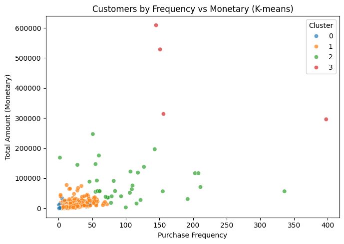
The goal of this project is to use the Online Retail II dataset to build a K-means model capable of revealing natural patterns in customer behavior, without relying on predefined labels or assumptions. My intention is to understand how customers group themselves based on their activity levels, spending behavior, and the time since their last purchase. Although this dataset comes from a retail environment, the behavioral logic behind it aligns closely with the type of analysis I care about in financial operations, especially accounts receivable, payment behavior, past-due patterns, and dispute generation.

The foundation of this analysis is the construction of the RFM table (Recency, Frequency, Monetary). These three metrics are not arbitrary; they summarize the core of customer behavior over time.

• Recency tells me how long it has been since the last transaction.
• Frequency captures how active the customer is.
• Monetary reflects the total value generated by that customer.

Despite their simplicity, these metrics contain enough information to model real behavioral patterns, making them ideal for clustering methods that depend on meaningful numerical structure rather than manual labels. In my work with financial and collections data, these concepts have direct analogues: days since last payment, number of payments or kept promises, and total billed or overdue amounts. That is why this project is more than just an academic exercise, it is a way to test, in a controlled environment, how a similar segmentation could later be applied to real operational processes.

I chose K-means because it fits perfectly with the problem I’m trying to solve. I’m not trying to predict an outcome or classify customers based on an existing rule; I’m trying to discover structure, identify natural groupings, and see whether the data genuinely contains distinct behavioral patterns. K-means is fast, interpretable, and robust enough for RFM-based datasets. It also forces me to think critically about the number of clusters that make sense for this population questions that mirror what I would ask when analyzing high-risk customers, prioritization strategies, or differentiated collection approaches.

The value I want from this model isn’t simply “clusters for the sake of clustering,” but actionable segments. I want to be able to say:

• these customers are active and valuable,
• these are showing early signs of churn,
• these spend a lot but transact irregularly.

From there, it becomes natural to think about targeted strategies: retention, operational adjustments, early-warning signals, or process redesign.

In short, this project is not just an exploration of K-means; it is a way to build the mental framework I need to later apply the same methodology to payment behavior, past-due evolution, disputes, and other financial processes where historical behavior reveals more than any intuition or manual filter. K-means is the right starting point because it helps me discover instead of assume, segment instead of label, and build a foundation for decisions rooted in real patterns, not opinions.

Importing the Core Libraries

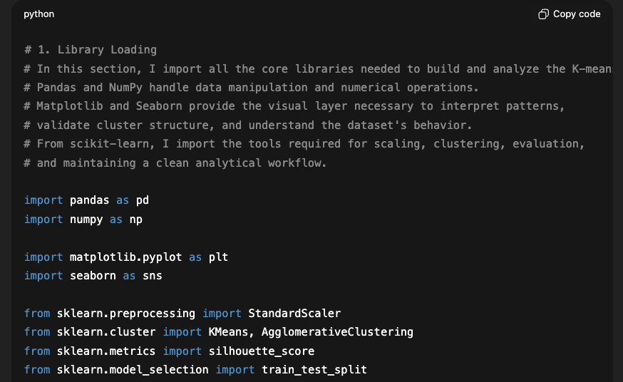
In this first section of the notebook, I import the essential libraries required for the analysis and for building the segmentation model. I use pandas and numpy as the foundation for manipulating and transforming the data; pandas allows me to work with tabular information in a way that feels like an advanced version of Excel, while numpy handles the numerical operations that support the machine learning algorithms.

For the visual component of the project, I incorporate matplotlib and seaborn, which make it possible to generate clear, comparable visualizations—crucial for interpreting the structure of the data, validating cluster quality, and identifying behavioral patterns.

Finally, I import the key tools from scikit-learn, including StandardScaler to normalize the RFM variables, clustering models such as KMeans and AgglomerativeClustering, the silhouette_score metric to evaluate cluster cohesion, and train_test_split to maintain a standard workflow structure, even if in this case it’s used more conceptually.

Together, this block of libraries establishes the technical ecosystem needed to process the data, build the model, and analyze the results in a rigorous and visually interpretable way.

Loading the Online Retail II Dataset

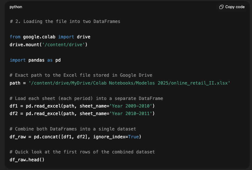
In this section of the project, I load the source file that contains the Online Retail II dataset. Since I am working in Google Colab, the first step is to mount Google Drive, which gives me access to the file stored in my personal repository. Once the environment is set up, I use pandas to read the Excel file, which includes two different sheets corresponding to two transactional periods (2009–2010 and 2010–2011).

Each sheet is loaded independently with pd.read_excel, explicitly specifying the sheet name to avoid any ambiguity. After that, I merge both DataFrames using pd.concat, creating a single homogeneous dataset called df_raw. This unified structure simplifies the analysis and eliminates the need to work with separate fragments.

Finally, I display the first few rows of the combined dataset to verify that both sheets were loaded and merged correctly. This validation step is important because it confirms that the dataset is complete and consistent before applying any transformations. Ensuring data integrity here sets the foundation for all the modeling steps that follow.

Preprocessing

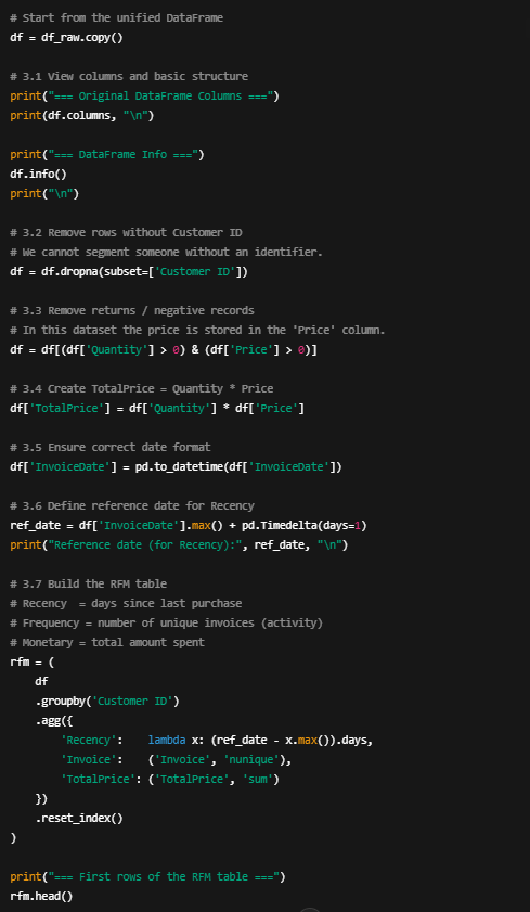
In this stage, I performed the initial cleaning and transformation of the dataset to prepare it for behavioral analysis and the later application of the K-means algorithm. I began by reviewing the overall structure of the DataFrame to confirm data types, identify missing values, and verify that the date column had been read correctly. This step is essential to prevent issues later on and to ensure that all computed metrics are based on consistent information.

I then removed all rows without a Customer ID, since a client without an identifier cannot be segmented or analyzed at the individual level. After that, I filtered out transactions representing returns or invalid records, specifically those with negative quantities or prices, to avoid distorting metrics such as total spending.

Next, I computed a new column called TotalPrice, calculated as Quantity × Price, which represents the exact value of each invoice line. I also standardized the date format for the InvoiceDate column and defined a reference date to compute the Recency variable, allowing me to determine how many days have passed since each customer’s last purchase.

Finally, I built the RFM table, grouping transactions by customer and calculating three key behavioral indicators:

• Recency (days since the last purchase),
• Frequency (number of unique invoices),
• Monetary (total amount spent).

This preprocessing step is fundamental because it transforms raw transactional history into a clean, compact behavioral representation—an ideal input for the clustering phase that follows

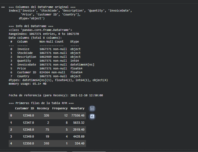
The results observed after the preprocessing stage confirm that the dataset was cleaned, filtered, and transformed correctly in order to build the RFM table. First, the original columns from the file are displayed, which allows me to verify that the variable names and types match the expected structure. Then, the df.info() report shows that the dataset contains more than one million valid transactions after removing entries without a Customer ID and those with inconsistent values. The columns have appropriate types: quantities and prices are numerical values, and the dates were successfully converted into the datetime64 format, which is essential for calculating the Recency variable. The reference date displayed, 2011-12-10, corresponds to one day after the last recorded transaction in the dataset and serves as the comparison point to determine how recent each customer’s last purchase was.

Finally, the first rows of the RFM table are shown, where each row represents a unique customer along with their three key indicators: Recency, Frequency, and Monetary. For example, the first customer (Customer ID 12346.0) has a Recency of 326 days, meaning they have gone almost a full year without purchasing. At the same time, they show a high Frequency (12 unique invoices) and a high Monetary value (over 77,000), suggesting they were a valuable customer who has recently become inactive. Other customers display different patterns: some purchase rarely but generate high value, others buy frequently but spend small amounts, and others show minimal interaction. These results demonstrate that the preprocessing pipeline worked correctly and transformed millions of individual transactions into a compact per-customer representation that accurately captures behavioral patterns. This RFM table will serve as the foundation for the K-means model to identify patterns and segment customers into homogeneous groups.

---

Split Data

For this unsupervised model, there is no need to split the data and instead train with the full dataset, since there is no target variable available to evaluate performance on a test set.

---

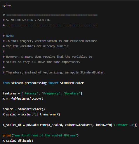
Vectorization

In the vectorization phase, I clarified that this step is not required for this project because the RFM data is already in numeric format and does not need any transformation to convert text or categorical values into vectors. However, since the K-means algorithm is highly sensitive to the scale of the variables, I performed a normalization process using StandardScaler. This ensures that Recency, Frequency, and Monetary all contribute proportionally to the distance calculations. In this way, I adapt the traditional “vectorization” step to what a numerical clustering model actually needs.

Search for the optimal number of clusters

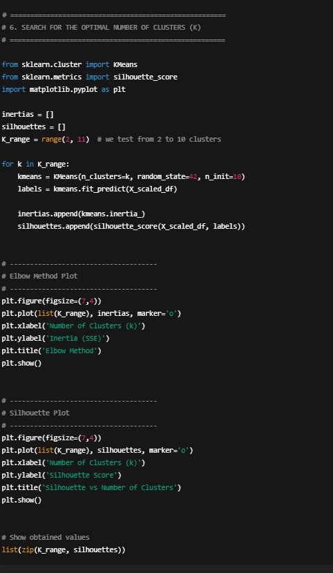
In this block of code, I perform a systematic search for the appropriate number of clusters for the K-means model. I begin by defining a range of possible values for k, from 2 to 10, since fewer than two clusters makes no sense and more than ten tends to produce overly fragmented groups. For each value of k, I train a K-means model using the scaled RFM data and compute two key metrics:

Inertia (SSE): measures how compact the clusters are; lower values indicate tighter groupings.
Silhouette Score: evaluates how well-separated the clusters are from one another; values closer to 1 are better.

Both metrics are stored in lists so they can be plotted afterward. I then generate two visualizations: the elbow method based on inertia, and the silhouette curve for each value of k. Finally, I print a list with all the computed values to compare them explicitly.

This process makes it possible to quantitatively evaluate which number of clusters strikes the right balance between internal compactness and separation across groups—an essential requirement for a meaningful segmentation.

Elbow Method

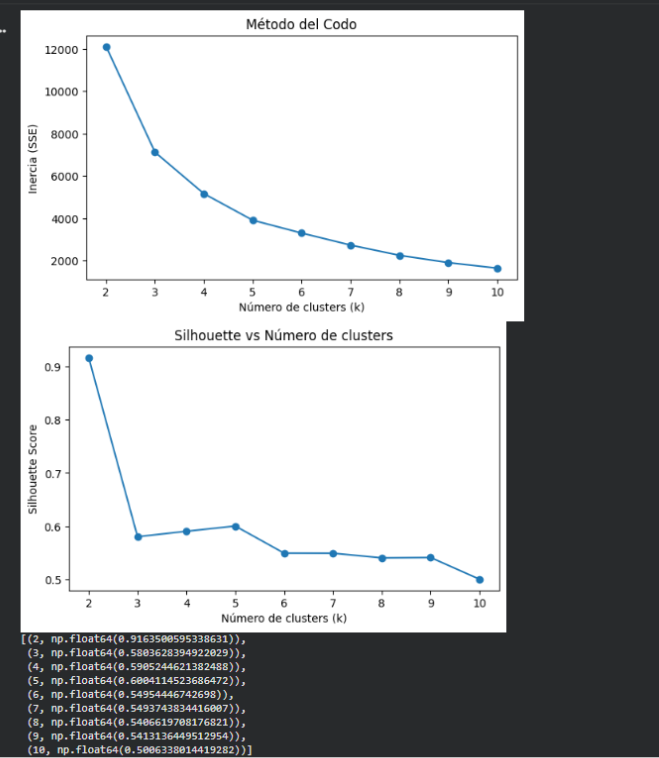
In the inertia plot, there is a sharp drop between K=2, K=3, and K=4. Starting at K=4, the curve begins to “flatten,” meaning that adding more clusters yields only marginal improvements. This pattern is exactly what defines the elbow method: a point where the benefit of increasing k decreases significantly.

This indicates that:

• K=4 and K=5 are the values where the structure stops improving substantially.
• Before that (K=2, K=3), there are still major gains.
• After that (K ≥ 6), the curve is almost flat.

---

Silhouette Score

In the second plot, the silhouette score shows:

• A very high value at K=2 (0.91), but this is not useful for meaningful segmentation, as it simply splits the data into two very broad groups.
• Starting from K=3, the silhouette stabilizes between 0.55 and 0.61.
• The highest useful value is K=4 (0.61).
• K=5 achieves a silhouette of 0.57, slightly lower.

The silhouette score helps validate how well differentiated the clusters are.

---

Conclusion Optimal K

After evaluating different values for the number of clusters using both the elbow method and the silhouette score, I conclude that the most appropriate range for segmenting this dataset is between K=4 and K=5.

The elbow method shows that the largest reduction in inertia happens between K=2 and K=4, and improvements become marginal beyond that point. The silhouette score identifies K=4 as the value with the best balance between cohesion and separation, reaching 0.61. Although K=2 has a very high silhouette, it produces an overly general segmentation. And while K=5 is also a valid option, its silhouette is slightly lower and represents more granular but not necessarily more stable clusters.

For these reasons, K=4 is considered the optimal value, though K=5 could be chosen intentionally if a more detailed segmentation is required.

Training K-means model

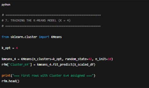
In this section, I train the K-means model using the optimal number of clusters previously selected through the elbow method and silhouette score analysis. Specifically, I configure the model to generate four clusters, which allows me to identify groups of customers with similar behaviors based on the scaled RFM metrics. The random_state parameter ensures reproducibility, and n_init=10 improves the algorithm’s stability by running multiple initializations.

I then fit the model using the scaled RFM data and assign each customer to a cluster, storing the result in the new Cluster_K4 column. This step establishes the foundation for the next phase, where I will interpret the profile of each group and analyze their relevance in terms of customer behavior.

Interpretation of the 4 clusters

Cluster 3 — “Ultra Active – Ultra High Value” (elite segment)

• Recency: ~3.5 days (bought extremely recently)
• Frequency: ~212 purchases (hyperactive)
• Monetary: ~436,835

This is the absolute top tier of the customer base—high-volume, high-frequency, extremely valuable clients.
Equivalent in AR to clients who pay constantly, generate massive revenue, and require VIP-level attention.

Typical profile:

• Large corporate buyers
• High-volume distributors
• Companies with recurring purchase orders

They are always top priority.

---

Cluster 2 — “Very Active – High Value”

• Recency: ~26 days (recent and active)
• Frequency: ~104 purchases
• Monetary: ~83,086

These are premium, consistent, high-value customers—not as extreme as Cluster 3, but clearly important.

Typical profile:

• High-volume but slightly less intense than Cluster 3
• Loyal and recurrent
• Strong purchasing behavior

In AR terms: high-value, reliable accounts.

---

Cluster 1 — “Moderately Active – Medium Ticket”

• Recency: ~67 days
• Frequency: ~7 purchases
• Monetary: ~3,009

This is the backbone of normal business operations.
They buy periodically, they return, but they don’t drive the majority of revenue.

Typical profile:

• Regular customers
• Stable relationship
• Low risk, low complexity

They’re not highly profitable, but they’re steady.

---

Cluster 0 — “Inactive – Low Value” (lost or nearly lost customers)

• Recency: ~463 days (inactive for over a year)
• Frequency: ~2 purchases
• Monetary: ~765

This is the lowest-value segment.
Equivalent in AR to small accounts with minimal strategic relevance.

Typical profile:

• Casual buyers
• One-time or trial customers
• Completely inactive customers

Not worth investing significant resources.

Cluster	Interpretation
3	Ultra VIP — hyperactive, extremely high value
2	Premium VIP — very active and high value
1	Regular customer — moderate activity, medium ticket
0	Inactive — low value, essentially lost

Cluster Interpretation

The K-means segmentation with K = 4 reveals four clearly differentiated customer groups.
Cluster 3 represents the most valuable and most active customers in the dataset recent buyers (3.5 days on average), with extremely high frequency (over 200 transactions) and exceptionally large monetary values.
Cluster 2 groups customers who are also very active and high value, though at more moderate levels compared to the top cluster.
Cluster 1 corresponds to regular customers with stable behavior, moderate frequency, and medium spending, effectively forming the operational backbone of the business.
Finally, Cluster 0 identifies inactive, low-value customers—those who have not purchased for over a year, have low ticket sizes, and show minimal historical interaction.

This segmentation captures meaningful behavioral patterns and allows for differentiated strategies across ultra-high-value clients, premium clients, regular customers, and those who are essentially lost.

Conclusion

In this project, I used the Online Retail II dataset to build a segmentation model based on clustering techniques, specifically K-means, with the goal of identifying behavioral patterns among customers using transactional metrics. The process began with extensive cleaning and structuring of the dataset to generate three fundamental variables: Recency, measuring the days since the last purchase Frequency, summarizing the number of distinct transactions and Monetary, representing the total amount spent by each customer. These three dimensions effectively synthesize purchasing behavior and allow for standardized comparison across customers. Once the RFM table was constructed, I normalized the variables to prevent differences in scale from distorting the analysis, since K-means relies directly on geometric distances.

Next, I evaluated different values of k to determine the optimal number of clusters. I used two complementary methods: the elbow method, which examines how inertia decreases as the number of clusters increases, and the silhouette score, which evaluates how well-separated the clusters are. Both methods indicated that the most reasonable values were within the 4–5 cluster range, confirming that these choices strike an appropriate balance between internal compactness and separation across segments. Based on this, I trained a K-means model with K = 4 and then with K = 5 to compare granularity and practical interpretability.

The model with K = 4 revealed four well-defined groups: a cluster of inactive, low-value customers; a cluster of regular customers with stable, moderate behavior; a cluster of highly active and valuable customers with significant spending; and an elite group of extremely active customers with very recent purchases, high frequency, and extraordinary monetary value. This segmentation not only captured the patterns present in the original data, but also produced a structure that is easy to interpret and directly applicable to real business scenarios. The key insight is that, although the model is trained on standardized values, the interpretation must rely on the original metrics, as they represent real behaviors such as days, amounts, and frequencies.

In retrospect, several aspects could be improved or enriched. First, incorporating additional variables—such as country, product type, channel, or seasonality would allow for richer, more commercially relevant segments. Second, the dataset includes returns and incomplete transactions; although these were partially filtered, a deeper analysis could improve model quality. Moreover, while RFM is powerful, it is inherently limited: it does not capture finer temporal relationships or sequential patterns that might reveal behaviors such as churn, growth, or risk. Another aspect worth exploring is the logarithmic transformation of the Monetary variable, which can sometimes improve clustering stability when the distribution has long tails.

Regarding the model itself, K-means worked well here, but it is not always the best method. K-means assumes spherical, balanced clusters an assumption that rarely holds in real-world data. Models like DBSCAN or HDBSCAN can detect density-based clusters and identify irregular shapes without requiring a predefined k, and they can flag “noise” customers, which is useful when atypical behaviors exist. Gaussian Mixture Models (GMM), on the other hand, allow elliptical clusters and overlapping distributions, capturing smoother transitions between customer profiles. In a more robust project, comparing these models against K-means would be valuable to validate whether the discovered structure is consistent or whether an alternative segmentation aligns more naturally with business reality.