1. predicting sentiment from amazon reviews
I’ve always been fascinated by how platforms try to understand what we like. Years ago, Netflix used a simple star-rating system to recommend movies and shows, and it felt almost magical that a handful of stars could shape your entire watchlist. Behind the scenes, they were likely running some kind of early recommendation or sentiment model, trying to guess what those stars really meant. Today they’ve moved on to likes and double-likes, but the core idea is still the same: turn human feedback into patterns a machine can learn from.
That idea is what inspired this project. Instead of ratings for shows, I wanted to explore the sentiment hidden inside Amazon product reviews. A five-star review doesn’t always mean “amazing,” and a one-star review doesn’t always mean “awful.” The real meaning is in the text, and with the right model, you can teach a machine to interpret that tone automatically.
For this project I wanted to create a simple, clean and fully reproducible sentiment analysis pipeline using real-world data. I picked a public dataset from Kaggle that contains thousands of Amazon reviews for unlocked mobile phones. It has only two useful fields, the review text and the rating, but that’s enough to turn it into a supervised learning problem. I grouped the ratings into positive, neutral and negative, and the goal is straightforward:
given a review, predict the sentiment behind it.
Instead of jumping straight into a fancy model, I decided to make the whole process transparent: load the data, clean it, convert the text into something a model can understand (TF-IDF), train different algorithms and compare how they behave. Nothing extreme, just real steps you would follow in any practical ML workflow.
I tested three classic models: a Decision Tree, a Random Forest and a LinearSVC. Each one has a very different personality. Trees try to split the data into rules, Random Forest tries to fix the weaknesses of a single tree, and SVM simply looks for the best boundary between the classes in a high-dimensional space. Same problem, three different ways of thinking.
My goal here is not to build the “ultimate” sentiment model, but to show how these algorithms react to real text and to highlight the gap between them. This is useful if you work with customer feedback, reviews, support tickets, disputes or any situation where the tone of a message matters. The code is simple, the steps are clear, and anyone can reproduce it on their own.
2. Dataset Overview (Kaggle: Amazon Unlocked Mobile Reviews)
Here’s a quick overview of the dataset I used for this project. The data comes from Kaggle’s Amazon Unlocked Mobile Reviews, a public dataset containing hundreds of thousands of real customer reviews for unlocked smartphones sold on Amazon.
The dataset includes around 400,000 reviews, each with a star rating and an open-text comment. For my pipeline, I only needed two columns:
- Rating (1 to 5 stars)
- Review Text
Every row represents one customer review written in natural language. The original rating system is numeric, so I transformed it into three sentiment classes to build a supervised learning problem:
- 1–2 stars → negative
- 3 stars → neutral
- 4–5 stars → positive
This mapping is simple, but it works surprisingly well. A star rating gives us a reliable proxy for the emotional tone of the review, and the text becomes the feature that the models learn from.
In the next steps of the pipeline, the text is cleaned, vectorized using TF-IDF, split into training and test sets, and then used to train three different classifiers. The dataset is large enough to create meaningful patterns, but still small enough to run smoothly in a typical Colab or laptop environment.
2. TOOLS AND LIBRARIES
Before building the sentiment analysis pipeline, the first step is to load the libraries that will be used throughout the project. First, NumPy and pandas handle basic data manipulation, and scikit-learn provides everything else I need: splitting the dataset, converting text into numeric features with TF IDF, training the machine learning models and evaluating their results. I also include a small line to hide warning messages so the notebook stays clean while running. With these imports, the whole workflow is ready to go and the rest of the project becomes straightforward.
import warnings
warnings.filterwarnings("ignore")   # hides unnecessary warning messages

import numpy as np                  # numerical operations and arrays
import pandas as pd                 # data loading and manipulation

from sklearn.model_selection import train_test_split   # splits data into train and test sets
from sklearn.feature_extraction.text import TfidfVectorizer  # converts text into numeric features
from sklearn.tree import DecisionTreeClassifier        # first ML model
from sklearn.ensemble import RandomForestClassifier    # second ML model
from sklearn.metrics import classification_report, accuracy_score  # evaluation metrics
from sklearn.svm import LinearSVC                      # third ML model (SVM)
3. DATA CLEANING AND PREPROCESSING
# Mount Google Drive to access the dataset stored there
from google.colab import drive
drive.mount("/content/drive")

# Read the CSV file from Drive into a pandas DataFrame
# Adjust the path if your file is in a different folder
dataSet = pd.read_csv(
    "/content/drive/MyDrive/Colab Notebooks/Amazon_Unlocked_Mobile.csv",
    header=0
)

# Preview the first rows to make sure the data loaded correctly
print(dataSet.head())

# Optionally, check the shape to see how many rows and columns we have
print("Shape:", dataSet.shape)
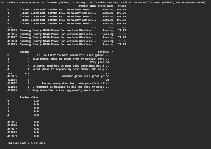
Before modeling, the first step is to load the dataset and take a quick look at what we are working with. I keep everything in Google Drive so I mount it inside Colab and read the CSV directly from there. The dataset contains several columns including product name, brand and price, but for this project I only care about two of them: the review text and the rating. The goal here is simply to load the raw data, verify that it was imported correctly and preview a few rows to understand its structure. This helps confirm that the text is clean enough to use, that the ratings are in the expected range from 1 to 5 and that there are no surprises in the file. Once I know the data is correctly loaded, I can move on to the actual preprocessing steps like selecting the relevant columns, handling missing values and creating the sentiment labels.
# Remove rows with missing values to avoid issues during training
dataSet.dropna(inplace=True)
# Create binary columns just to visualize how each rating maps to the new labels
# 1 if rating is 4 or 5, otherwise 0
dataSet["Positively_Rated"] = dataSet["Rating"].apply(lambda r: 1 if r >= 4 else 0)
# 1 if rating is exactly 3, otherwise 0
dataSet["Neutral_Rated"] = dataSet["Rating"].apply(lambda r: 1 if r == 3 else 0)
# 1 if rating is 1 or 2, otherwise 0
dataSet["Poorly_Rated"] = dataSet["Rating"].apply(lambda r: 1 if r <= 2 else 0)
# Function to map numeric ratings into a 3-class sentiment label
def classify_sentiment(r):
if r >= 4:
return "positive"
elif r == 3:
return "neutral"
else:
return "negative"
# Apply the function to create a final sentiment column
dataSet["Sentiment"] = dataSet["Rating"].apply(classify_sentiment)
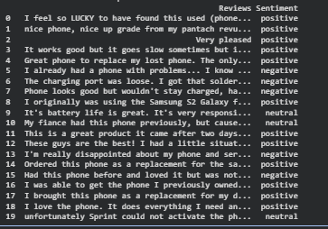
# Show intermediate columns for clarity and documentation
misDatos = dataSet[["Reviews", "Rating",
"Positively_Rated", "Neutral_Rated", "Poorly_Rated"]]
print("Preview of intermediate columns:")
print(misDatos.head(20))
# Final dataset used for training (only review text and the sentiment label)
finalData = dataSet[["Reviews", "Sentiment"]]
print("Preview of the final dataset:")
print(finalData.head(20))
Once the raw data is loaded, the next step is to clean it and create the labels that the model will learn from. I start by removing any rows with missing values so the training process stays simple and predictable. The dataset originally uses numeric ratings from 1 to 5, so I created a set of helper columns that show how each rating maps into negative, neutral or positive sentiment. This part is not required for the model but it helps visualize what is happening behind the scenes.
After that, I define a small function that groups the ratings into three classes: 4 and 5 become positive, 3 becomes neutral and 1 or 2 becomes negative. This gives me a clean sentiment column that will be used as the target variable. I show the intermediate columns for transparency and then reduce the dataset to only the two fields I actually need for modeling: the review text and the final sentiment label. From here the data is ready to be split into training and test sets and passed into the vectorization step.
4. Traing Test split
Before training any model, I split the data into a training set and a test set. I use 75 percent of the reviews for training and keep the remaining 25 percent aside for evaluation. The idea is simple: the model is only allowed to see the training data while it learns, and the test data is treated as completely new information. This gives a much more honest estimate of how the model will behave in the real world.
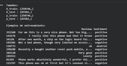
In this step I separate the input features and the target variable. The X variable holds only the raw review text, and y contains the final sentiment label with the three classes: positive, neutral and negative. I use scikit learn’s train_test_split function with the stratify option so that the proportion of each class is similar in both sets. With this configuration I end up with around 257,000 reviews for training and 83,000 for testing, which is more than enough for the models to learn meaningful patterns. Printing the shapes and a few sample rows is a quick sanity check that confirms the split worked as expected and that the sentiment labels still align correctly with the review text.
from sklearn.model_selection import train_test_split

# Proportion of data used for training
train_size = 0.75
test_size = 1 - train_size

# Input features (X) and target variable (y)
# X will contain only the review text
# y will contain the 3-class sentiment label
X = finalData["Reviews"]
y = finalData["Sentiment"]

# Stratified split so that the class distribution
# (positive, neutral, negative) is similar in both sets
X_train, X_test, y_train, y_test = train_test_split(
    X,
    y,
    test_size=test_size,
    random_state=42,   # for reproducible results
    stratify=y        # keep class proportions
)

# Show the shapes to verify the split
print("Sizes:")
print("X_train:", X_train.shape)
print("X_test :", X_test.shape)
print("y_train:", y_train.shape)
print("y_test :", y_test.shape)

# Show a few training examples
print("\nTraining examples:")
print(pd.concat([X_train.head(10), y_train.head(10)], axis=1))
5. tf idf vECTORIZATION
The next step in the pipeline is to turn the raw text into something a machine learning model can actually use. Models cannot work with words directly, so I use TF IDF to convert every review into a numeric vector. TF IDF gives more weight to words that appear often in a specific review but not too often across the entire dataset. That means words like “broken”, “excellent”, “refund” or “love” carry more meaning than very common words like “phone”, “it” or “this”. I fit the TF IDF vectorizer only on the training set, then apply the transformation to both training and test data. This avoids leaking information from the test set into the model. The final result is a large sparse matrix where each row represents a review and each column represents a word in the vocabulary. These vectors become the actual input for the three models I train in the next sections. Even though TF IDF is simple compared to modern embedding methods, it is still one of the most reliable ways to handle text classification and works remarkably well for sentiment analysis.
from sklearn.feature_extraction.text import TfidfVectorizer

# Create the TF-IDF vectorizer
vectorizer = TfidfVectorizer(
    stop_words='english',  # remove English stopwords
    min_df=5,              # ignore words that appear in fewer than 5 reviews
    max_df=0.8,            # ignore words that appear in more than 80% of the reviews
    sublinear_tf=True,     # use log(1 + tf) to avoid overweighting repeated words
    use_idf=True           # enable the IDF component
)

# Fit only on the training set and transform
X_train_vec = vectorizer.fit_transform(X_train)
X_test_vec  = vectorizer.transform(X_test)

print("Shape of the TF-IDF matrices:")
print("X_train_vec:", X_train_vec.shape)
print("X_test_vec :", X_test_vec.shape)

6. MODELS: decision tree
The first model I tested was a Decision Tree. It is one of the most intuitive algorithms, since it essentially learns a set of if else rules that split the data into smaller and smaller groups. In this case the tree receives the TF IDF vectors as input and tries to separate the three sentiment classes based on the words that appear in each review. I limited the depth of the tree to 10 levels so it does not grow too large or overfit the training data completely.
from sklearn.tree import DecisionTreeClassifier
from sklearn.metrics import accuracy_score, classification_report

# Model 1: Decision Tree
# max_depth limits how deep the tree can grow
# random_state makes the result reproducible
dt_clf = DecisionTreeClassifier(max_depth=10, random_state=42)

# Train the model on the TF IDF training vectors
dt_clf.fit(X_train_vec, y_train)

# Make predictions on the test set
dt_pred = dt_clf.predict(X_test_vec)

# Print accuracy and a full classification report
print("=== Decision Tree ===")
print("Accuracy:", accuracy_score(y_test, dt_pred))
print(classification_report(y_test, dt_pred))
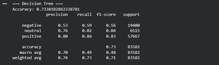
On the test set the Decision Tree reached an overall accuracy of about 73 percent. Looking at the classification report gives a clearer picture of how it behaves. For the positive class, which is the largest group, the model performs reasonably well, with a precision of 0.80, a recall of 0.86 and an F1 score of 0.83. This means that most positive reviews are detected correctly and not too many non positive reviews are mislabeled as positive. The negative class is weaker, with a precision of 0.53 and recall of 0.59, which shows that the model misses a good portion of the negative reviews and is not very confident when predicting that label.
The real problem appears in the neutral class. Even though the precision is 0.76, the recall drops to 0.02 and the F1 score is only 0.04. In practice this means the tree almost never predicts the neutral label. When it does, it is usually correct, but it predicts it so rarely that the model is basically ignoring that class. Most neutral reviews are being pushed into positive or negative. This is a common issue with decision trees on high dimensional text data, especially when the classes are imbalanced and one class is much smaller than the others. The macro averages confirm this behavior, with a macro F1 of 0.48, which is much lower than the weighted F1 of 0.71 that is dominated by the positive class.
As a baseline model, the Decision Tree is useful because it gives a simple reference point and a clear view of how the data is being split, but the metrics already suggest that we will need something more robust to handle the three class sentiment problem, especially if we care about capturing neutral reviews correctly.
7. MODELS: RANDOM FOREST
The second model I tested was a Random Forest, which is basically an ensemble of multiple decision trees working together. The idea is that instead of relying on a single tree and its biases, the model builds many smaller trees and lets them vote on the final prediction. This usually makes the model more stable and less sensitive to noise. I limited the depth of each tree to prevent overfitting and allowed the model to use a large number of features since TF IDF generates thousands of them.
from sklearn.ensemble import RandomForestClassifier
from sklearn.metrics import accuracy_score, classification_report

# Model 2: Random Forest
# n_estimators is the number of trees in the forest
# max_depth controls how deep each tree can grow
# max_features limits how many features are considered at each split
# n_jobs=-1 allows the model to use all CPU cores
rf_clf = RandomForestClassifier(
    n_estimators=100,
    max_depth=6,
    max_features=5000,
    random_state=42,
    n_jobs=-1
)

# Train the model on the TF-IDF vectors
rf_clf.fit(X_train_vec, y_train)

# Predict on the test set
rf_pred = rf_clf.predict(X_test_vec)

# Print accuracy and classification report
print("=== Random Forest ===")
print("Accuracy:", accuracy_score(y_test, rf_pred))
print(classification_report(y_test, rf_pred))
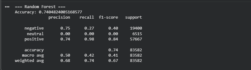
On the test data, the Random Forest reached an accuracy of about 74 percent, which is very similar to the Decision Tree. At first glance this might suggest an improvement, but the classification report tells another story. The model performs extremely well on the positive class, with a recall of 0.98 and an F1 score of 0.84. This means it correctly identifies almost every positive review. The downside is that the model becomes heavily biased toward predicting that same class.
For the negative class, the results drop significantly. Precision is 0.75, meaning the model is usually correct when it predicts negative, but recall is only 0.27, so it misses most of the actual negative reviews. This shows that even with a combination of trees, the model is struggling to capture the smaller negative class.
The situation is most visible in the neutral class, where the model reaches precision 0.00, recall 0.00 and F1 0.00. This tells us the model never predicts a neutral label at all. It sends almost everything to either positive or negative. The neutral class is the smallest group, and Random Forest tends to ignore underrepresented classes when the feature space is very large, which is typical for TF IDF text models.
The macro average F1 score of 0.42 highlights this imbalance. Even though the weighted average F1 score looks decent at 0.67, this value is dominated by the positive class and hides the model’s inability to detect neutrals.
Overall, the Random Forest performs better than the Decision Tree on positive reviews but completely fails to capture the neutral class. This makes it unsuitable for a three class sentiment problem unless additional techniques like class balancing or better text representations are introduced.
8. MODELS: LINEAR SVC (Linear support vector machine)
The third model I trained was a Linear Support Vector Machine, which is one of the strongest baselines for text classification. Unlike decision trees or random forests, Linear SVC works very well in high dimensional spaces like TF IDF matrices. The model tries to find the best possible boundary between the three sentiment classes by maximizing separation in the feature space. This makes it particularly good at capturing subtle patterns in text, where many words contribute small amounts of information
from sklearn.svm import LinearSVC
from sklearn.metrics import accuracy_score, classification_report

# Model 3: Linear SVC (linear Support Vector Machine)
# random_state ensures reproducible results
svm_clf = LinearSVC(random_state=42)

# Train the model using the TF-IDF vectors
svm_clf.fit(X_train_vec, y_train)

# Predict on the test set
svm_pred = svm_clf.predict(X_test_vec)

# Print accuracy and classification report
print("=== LinearSVC (Linear SVM) ===")
print("Accuracy:", accuracy_score(y_test, svm_pred))
print(classification_report(y_test, svm_pred))
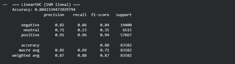
The performance of Linear SVC clearly stands out. The overall accuracy reaches 88 percent, which is a significant improvement over the previous models. But the real advantage appears when looking at precision, recall and F1 scores across the three classes. The positive class performs exceptionally well, with an F1 score of 0.94, meaning the model captures almost all positive reviews correctly. For the negative class the performance is also strong, with a precision of 0.82, recall of 0.86 and an F1 score of 0.84, much better than what the Decision Tree and Random Forest were able to achieve.
The most important gain happens in the neutral class. While the previous models practically ignored it, Linear SVC manages to give it meaningful predictions. Precision reaches 0.71, recall rises to 0.23 and the F1 score increases to 0.35. This is still not perfect and the class remains the hardest to predict, but compared to the recall of 0.02 or 0.00 seen before, this is a huge improvement. Linear SVC is finally able to detect a noticeable portion of the neutral reviews.
The macro average F1 score of 0.71 reflects a much more balanced performance across classes, and the weighted average of 0.87 confirms that the model handles the entire dataset well. In short, Linear SVC is by far the best model for this problem. It leverages the large vocabulary created by TF IDF and captures both strong and subtle patterns in the text, making it the most reliable option for a multi class sentiment classification task.
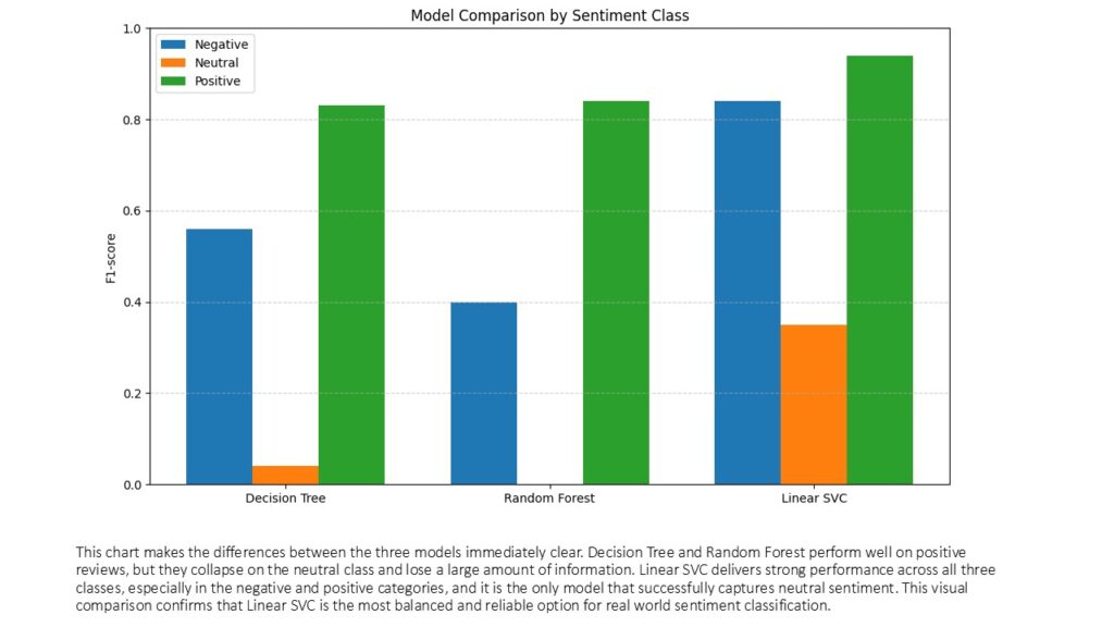
9. results and comparison
After training the three models under the exact same conditions, the differences in performance become very clear. The Decision Tree and Random Forest models struggle with the structure of text data. Even though they achieve acceptable accuracy when averaged across the entire test set, they fail to correctly identify the minority classes, especially the neutral sentiment. Both models are heavily biased toward predicting the majority class, which in this dataset is positive reviews.
The Linear SVC model, on the other hand, takes full advantage of the high dimensional TF IDF vectors. It learns far more expressive boundaries and handles both majority and minority classes much better. Not only does it reach the highest accuracy, but it also consistently improves precision, recall and F1 score across all sentiment labels. Most importantly, it is the only model that truly recognizes the neutral class in a meaningful way.
From a practical standpoint, Linear SVC is the only model among the three that is reliable enough to use in a real world setting. Decision Trees can be useful for understanding simple decision boundaries, and Random Forest improves stability, but neither captures the complexity of natural language as effectively as a linear SVM.
| Model | Accuracy | Negative F1 | Neutral F1 | Positive F1 | Macro F1 | Notes |
|---|
| Decision Tree | 0.73 | 0.56 | 0.04 | 0.83 | 0.48 | Almost ignores neutral class |
| Random Forest | 0.74 | 0.40 | 0.00 | 0.84 | 0.41 | Predicts neutral as zero |
| Linear SVC | 0.88 | 0.84 | 0.35 | 0.94 | 0.71 | Best overall performance |
10. FINAL INTERPRETATION
Linear SVC wins by a large margin because it is naturally suited for large sparse feature spaces created by TF IDF.
Decision Tree and Random Forest collapse on the neutral class, showing that tree based models have trouble handling subtle sentiment distinctions when most words appear in many reviews.
Accuracy alone is misleading. If we only looked at accuracy, the three models seem close, but the class level metrics tell the real story.
For real world sentiment analysis, Linear SVC is the clear choice, unless we move toward deep learning models or embeddings such as BERT.
11. CONCLUSION
Working with the Amazon Unlocked Mobile Reviews dataset gave me a good opportunity to see how far a traditional machine learning pipeline can go when dealing with real text written by real customers. The dataset is large, noisy and unbalanced, and that alone tells us something important. Most people tend to write reviews only when the experience was either very good or very bad, and far fewer take the time to leave a neutral comment. That imbalance directly affected the models. Even though the Linear SVC reached an accuracy close to 88 percent, the performance varies across the three sentiment classes. The model is extremely good at identifying positive reviews and solid at capturing negative ones. The neutral class is still the most challenging because the language used in those comments is often vague and the number of neutral examples is much smaller. In other words, the 88 percent accuracy is not a single truth, it is an average that hides the fact that some sentiments are easier to detect than others.
If a business user had to work with these results, the interpretation would depend on the goal. For example, if the objective is to understand overall customer satisfaction or to decide which products deserve more inventory, the model is already useful. It can automatically highlight products that accumulate strong positive reviews and quickly detect those where negative sentiment is rising. This type of signal can support decisions around stock levels, promotions, supplier negotiations, or prioritizing customer service interventions. Even at 88 percent accuracy, the model is far faster and more consistent than reading thousands of reviews manually. What it cannot do yet is treat the neutral category with the same level of confidence, so any decision that depends heavily on subtle or borderline sentiment would require additional analysis.
Sentiment analysis also has many uses beyond product reviews. It can support customer support teams by scoring incoming messages, help detect unhappy clients before they churn, classify social media conversations, or analyze feedback from surveys. In all these cases, this is a supervised model because we start with a labeled dataset; the target variable already exists, and the model learns the relationship between the text and the sentiment. Without labeled data we would need a different approach, probably an unsupervised method, but that would not give us the same clarity or control over the output.
Looking back, there are several things we could try as next steps. We could rebalance the dataset to give more weight to the neutral class, tune the TF IDF parameters, or explore additional models like logistic regression, which is known to work extremely well on TF IDF features. Another idea is to experiment with n grams or adjust how the vocabulary is constructed. All these remain within the limits of classic machine learning, without jumping into deep learning or transformer models. They would likely improve the model’s balance across classes, especially for the neutral category.
Overall, the project achieved what I intended when I started. I wanted to take a real dataset, build a clean pipeline around it, compare different models and understand not only which one performs best but also why. I also wanted an example that reflects how machine learning looks in practice, with the good parts and the limitations. The results remind me of something simple but valuable: even a straightforward model, when trained correctly, can extract meaningful insight from raw text and help people make better decisions. That was the motivation behind this experiment, and I think the final outcome stays aligned with that goal.
Leave a Reply