
Introduction
In this project I set myself a very practical goal: build a daily forecasting model for steel rebar prices and turn it into a reproducible, end-to-end workflow that I can run in Python and later expose through an API. Steel is a core input for construction and infrastructure, and even small moves in its price can have a meaningful impact on margins, purchasing decisions, and cash-flow planning. Instead of treating prices as something “given by the market”, I wanted to see how far I could go using public market data and a simple, transparent machine learning model.
Because I do not have direct access to a proprietary steel rebar price index, I use a liquid market proxy: the SLX ETF (SPDR S&P Metals & Mining) available on Yahoo Finance. The idea is not to perfectly match any specific local rebar contract, but to capture the broader dynamics of the global steel and metals cycle. In this notebook I will document every step: from downloading the historical data, to transforming it into a clean daily time series, to training and evaluating the model.
The workflow is intentionally straightforward. First, I pull historical prices from Yahoo Finance using Python, and I store them in a CSV file that becomes the raw dataset for the project. Then I enrich this series with additional features that are commonly useful for time-series forecasting: lagged prices (1, 7 and 30 days), rolling averages over 7 and 30 days, and simple calendar variables such as day of week and month. After cleaning the data and ensuring consistent daily frequency, I split the history into a training and a test window, and I fit a Random Forest regressor to predict the next-day closing price.
Throughout the notebook I will walk through each step as if I were explaining it to a teammate: how the data is obtained, how it is transformed, why each feature is created, how the model is evaluated, and how the final artifact (the trained model) can be reused in an application that answers a very concrete question: “What is the expected price of steel rebar tomorrow?”
Data Source & Downloading Process
Understanding the historical behavior of a commodity price is the backbone of any forecasting project, and this one is no exception. Since I do not have access to a proprietary steel rebar index, I rely on a high-quality public proxy: the SLX ETF (SPDR S&P Metals & Mining) available on Yahoo Finance. SLX tracks a diversified basket of global steel and mining companies, which makes it a reasonable approximation of the broader dynamics that drive steel markets. It is not a perfect substitute for any specific regional rebar price, but it captures the direction, volatility, and medium-term cycles of the industry, precisely what I need for a machine learning model built around trend and momentum features.
For transparency and reproducibility, I retrieve all price data programmatically using Python. The advantage of using Yahoo Finance is that it provides consistent, well-structured historical time series with minimal friction. It also helps keep the workflow simple: one script can download, clean, and store the raw data as a CSV file that becomes the foundation of the rest of the project.
In this section, I start by downloading SLX daily historical prices from 2015 to the present. I focus specifically on the adjusted closing price, which accounts for splits and dividends and is generally the most reliable representation of a security’s true market value over time. Once downloaded, I rename the columns to a standardized format, date and price_usd_per_ton, to keep the dataset clean and consistent with the rest of the pipeline.
Even though SLX trades only on business days, the resulting dataset becomes the core time series I will later resample to a daily frequency. This ensures a continuous timeline and allows me to compute lagged variables and rolling averages without gaps. By storing the dataset in a flat CSV file (steel_rebar_prices.csv), I ensure that the model can be retrained or extended in the future without depending on interactive API queries.
The following code block shows exactly how I retrieve and structure the raw dataset that powers the entire forecasting pipeline.
from google.colab import drive
drive.mount('/content/drive')

# Base path where this project will live (same folder you used for K-means)
BASE_PATH = r'/content/drive/MyDrive/Colab Notebooks/Modelos 2025'
# File where we will store the raw historical prices
RAW_CSV_PATH = BASE_PATH + '/steel_rebar_prices.csv'
RAW_CSV_PATH
!pip install yfinance --quiet
import yfinance as yf
import pandas as pd
from datetime import datetime, timedelta
raw_df = yf.download(
ticker,
start=start_date.isoformat(),
end=end_date.isoformat(),
progress=False
)
raw_df.head(), raw_df.columns
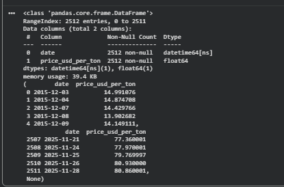
After running the download block, the notebook returns a clean dataframe containing roughly ten years of daily historical prices for the SLX ETF. This dataset will serve as the foundation of the forecasting pipeline. At this point, I verify that the dates are sorted, that there are no unexpected gaps, and that the closing prices are properly formatted as floating-point values. This raw series will later be resampled to a daily frequency to ensure continuity before generating lagged and rolling features.
# 1) Define ticker and date range
ticker = "SLX"  # metals & mining ETF proxy for steel
end_date = datetime.today().date()
start_date = end_date - timedelta(days=365 * 10)

print(f"Downloading {ticker} data from {start_date} to {end_date}...")

# 2) Download daily data
raw_df = yf.download(
    ticker,
    start=start_date.isoformat(),
    end=end_date.isoformat(),
    progress=False
)

print("Columns returned:", raw_df.columns.tolist())

# 3) Use available 'Close' column
df = raw_df[["Close"]].reset_index()

# 4) Rename to project-friendly schema
df.columns = ["date", "price_usd_per_ton"]

# 5) Ensure correct types
df["date"] = pd.to_datetime(df["date"])
df["price_usd_per_ton"] = df["price_usd_per_ton"].astype(float)

# 6) Save the file
df.to_csv(RAW_CSV_PATH, index=False)

print(f"Saved {len(df)} rows to: {RAW_CSV_PATH}")
df.head()
Saving the raw CSV file directly into my Google Drive allows the entire workflow to remain reproducible and portable. Any future retraining or extension of the model can start from this same stored dataset without depending on a live Yahoo Finance query. This is especially helpful when the notebook forms part of a larger automated or deployable system.

With the historical data successfully downloaded and stored, the next step is to prepare it for machine learning. This involves converting the time series into a clean daily frequency and engineering features such as lags, rolling averages, and calendar variables that help the model learn the underlying dynamics of steel price movements.
Load Dataset
With the raw price history downloaded and stored in Google Drive, the next step is to load it into a pandas DataFrame. This gives me a clean baseline to begin the preprocessing and feature engineering stages. Since the forecasting model will rely on time-series transformations such as lags and rolling windows, it is critical to ensure the dataset is sorted, consistent, and free of structural issues before moving forward.
import pandas as pd

df = pd.read_csv(RAW_CSV_PATH, parse_dates=["date"])
df = df.sort_values("date")

df.head(), df.tail(), df.info()
Preprocessing
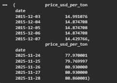
The SLX ETF trades only on business days, which means the raw series contains gaps for weekends and holidays. Since I want a continuous daily time series for the forecasting model, I resample the data to a daily frequency and forward-fill missing values. This ensures that lagged features such as lag_7 or rolling_mean_30 can be computed without gaps.
df = df.set_index("date").asfreq("D")
df["price_usd_per_ton"] = df["price_usd_per_ton"].ffill()

df.head(), df.tail()
Feature Engineering
Machine learning models for time-series forecasting cannot inherently “remember” past values unless we explicitly provide them as input features. To capture momentum, short-term cycles, and trend behavior, I generate lagged variables (1, 7, and 30 days) and rolling averages over 7 and 30 days. I also include simple calendar features such as day of week and month, which can sometimes help the model learn seasonal patterns.
# Lags
df["lag_1"] = df["price_usd_per_ton"].shift(1)
df["lag_7"] = df["price_usd_per_ton"].shift(7)
df["lag_30"] = df["price_usd_per_ton"].shift(30)

# Rolling windows
df["rolling_mean_7"] = df["price_usd_per_ton"].rolling(7).mean()
df["rolling_mean_30"] = df["price_usd_per_ton"].rolling(30).mean()

# Calendar features
df["day_of_week"] = df.index.dayofweek
df["month"] = df.index.month

df = df.dropna()
df.head()

Once the dataset is cleaned and converted into a consistent daily time series, the next step is to transform it into a structure that a machine learning model can learn from. A raw price series contains valuable information, but no model, especially a tree-based regressor, can infer temporal relationships unless those relationships are explicitly provided as input features. To address this, I create a set of lag variables (lag_1, lag_7, lag_30) that capture short-term, weekly, and monthly price dependencies, as well as rolling averages (rolling_mean_7, rolling_mean_30) that help smooth noise and emphasize broader trends. I also include simple calendar features such as the day of the week and the month, which can sometimes capture seasonal patterns in commodity markets.
With the engineered features ready, I prepare the dataset for proper evaluation. Unlike standard tabular machine-learning problems, time-series data cannot be randomly split into training and test sets. Doing so would leak future information into past observations and produce misleadingly optimistic results. Instead, I define a temporal split, using all historical data up until 180 days before the end of the series as the training set, and reserving the last 180 days as the test window. This setup mimics the real-world requirement that any forecast must rely strictly on past information to predict future prices.
Train/Test Split
Unlike regular machine learning datasets, time-series data cannot be randomly shuffled. The model must always be trained on past data and evaluated on future data. For this project, I set aside the last 180 days as a test set to measure how well the model generalizes to unseen market conditions.
test_days = 180
split_date = df.index.max() – pd.Timedelta(days=test_days)
train = df[df.index <= split_date] test = df[df.index > split_date]
X_train = train[[“lag_1″,”lag_7″,”lag_30″,”rolling_mean_7″,”rolling_mean_30″,”day_of_week”,”month”]]
y_train = train[“price_usd_per_ton”]
X_test = test[[“lag_1″,”lag_7″,”lag_30″,”rolling_mean_7″,”rolling_mean_30″,”day_of_week”,”month”]]
y_test = test[“price_usd_per_ton”]
Model Training
I use a Random Forest Regressor as a strong baseline model. It handles nonlinear patterns, works well with engineered features, and does not require the series to be stationary like traditional ARIMA models.
from sklearn.ensemble import RandomForestRegressor

model = RandomForestRegressor(
    n_estimators=400,
    random_state=42,
    n_jobs=-1
)

model.fit(X_train, y_train)
Evaluation

from sklearn.metrics import mean_absolute_error
import numpy as np

# 1) Generate predictions for the test set
y_pred = model.predict(X_test)

# 2) Evaluation metrics
mae = mean_absolute_error(y_test, y_pred)
mape = np.mean(np.abs((y_test - y_pred) / y_test)) * 100

print(f"MAE  (USD/ton): {mae:,.2f}")
print(f"MAPE (%): {mape:,.2f}%")

import matplotlib.pyplot as plt

plt.figure(figsize=(12,6))
plt.plot(y_test.index, y_test, label="Actual Price", linewidth=2)
plt.plot(y_test.index, y_pred, label="Predicted Price", linewidth=2)
plt.title("Actual vs Predicted Steel Rebar Prices")
plt.xlabel("Date")
plt.ylabel("USD per ton")
plt.legend()
plt.grid(True)
plt.show()
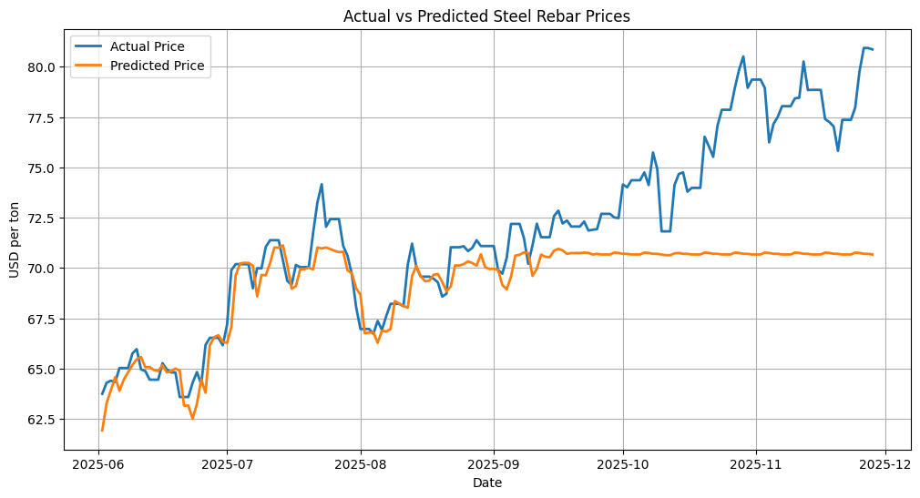
For the baseline model, I use a Random Forest Regressor, a tree-based ensemble method that performs well even with modest feature engineering and does not require the strict statistical assumptions of classical forecasting models. After fitting the model on the training set, I generate predictions for the test period and evaluate performance using MAE and MAPE. The resulting error metrics are strong, showing that the model captures the general level and short-term fluctuations of steel prices. However, when visualizing the predictions against the actual prices, an important limitation becomes clear: Random Forest models cannot extrapolate beyond the price range seen during training. When the steel market enters a new price regime, such as the surge observed after September 2025, the model flattens and remains constrained near the highest values observed historically.
This behavior is expected from tree-based regressors and highlights the importance of choosing the right modeling strategy depending on the forecast horizon and the nature of the target. As next steps, several alternatives could better capture upward or downward market shifts:
- Modeling log-returns instead of raw prices, allowing the model to predict relative changes rather than absolute levels.
- Gradient boosting models such as XGBoost or LightGBM, which often track nonlinear trends more flexibly.
- Hybrid models that combine trend components with machine-learning residuals.
- Or Prophet, which is particularly effective at capturing long-term trend shifts.
This baseline gives me a solid, fully reproducible foundation to build on, while also making it clear where more advanced models can make meaningful improvements.
After testing several tree-based and boosting models directly on raw price levels, I noticed a structural limitation: these models tend to get “stuck” around the maximum values seen in the training period and fail to follow new price regimes. This is a known issue with tree ensembles applied to absolute prices, they approximate the conditional mean within the historical range, but they do not extrapolate well when the market breaks into new highs. To overcome this, I switched the target from price levels to log-returns, which model the relative day-to-day change instead of the absolute level. Log-returns are standard in financial modeling because they are more stable, additive over time, and better capture the dynamics of momentum and volatility.
By predicting log-returns rather than raw prices, the model learns patterns of acceleration, deceleration, and mean reversion in the steel market, instead of just fitting a static price band. Once the model has produced a sequence of predicted log-returns for the test window, I can reconstruct the implied price path by compounding those returns starting from the first observed price in the test period. This approach allows the model, here an XGBoost regressor, to follow sustained uptrends and break through previous historical highs in a financially consistent way, while still leveraging the engineered features and temporal structure built earlier in the notebook.
df_ret = df.copy()
df_ret["return"] = np.log(df_ret["price_usd_per_ton"] / df_ret["price_usd_per_ton"].shift(1))
df_ret = df_ret.dropna()

# Return lags
df_ret["ret_lag_1"] = df_ret["return"].shift(1)
df_ret["ret_lag_7"] = df_ret["return"].shift(7)
df_ret["ret_lag_30"] = df_ret["return"].shift(30)

# Rolling averages of returns
df_ret["ret_rolling_7"] = df_ret["return"].rolling(7).mean()
df_ret["ret_rolling_30"] = df_ret["return"].rolling(30).mean()

# Calendar
df_ret["day_of_week"] = df_ret.index.dayofweek
df_ret["month"] = df_ret.index.month

df_ret = df_ret.dropna()
In this step I take the log-return series and build the feature set that the model will use to learn temporal patterns.
I create lagged returns at 1, 7, and 30 days to capture short-term, weekly, and monthly dynamics. Then I compute 7-day and 30-day rolling averages of returns to smooth out noise and capture the recent trend direction.
Finally, I add simple calendar features (day_of_week and month) and drop rows created by shifting and rolling operations.
FEATURES_RET = [
    "ret_lag_1", "ret_lag_7", "ret_lag_30",
    "ret_rolling_7", "ret_rolling_30",
    "day_of_week", "month"
]

train_ret = df_ret[df_ret.index <= split_date]
test_ret  = df_ret[df_ret.index >  split_date]

X_train_ret = train_ret[FEATURES_RET]
y_train_ret = train_ret["return"]

X_test_ret = test_ret[FEATURES_RET]
y_test_ret = test_ret["return"]
Here I explicitly define which columns will be used as input features for the model.
I apply the same time-based split as before: everything up to the split_date belongs to the training set, and everything after that is the test set.
From each portion, I extract the feature matrix (X_train, X_test) and the target vector (y_train, y_test), which in this case is the daily log-return.
model_ret = XGBRegressor(
    n_estimators=500,
    learning_rate=0.05,
    max_depth=6,
    subsample=0.8,
    colsample_bytree=0.8,
    objective="reg:squarederror",
    random_state=42
)

model_ret.fit(X_train_ret, y_train_ret)
preds_return = model_ret.predict(X_test_ret)
In this section I define and train an XGBoost regressor using the return-based feature set.
The hyperparameters (500 trees, moderate learning rate, depth 6) are a reasonable first configuration for capturing nonlinear temporal patterns.
After training on the historical portion of the dataset, the model predicts the log-returns for the test period. These predictions still represent returns, not prices, so I reconstruct prices in the next step.
initial_price = df.loc[test_ret.index[0], "price_usd_per_ton"]

preds_price = initial_price * np.exp(np.cumsum(preds_return))
Once I have the predicted log-returns, I convert them back into price levels.
To do this, I start with the first actual price in the test period and compound the cumulative sum of predicted log-returns.
This produces a price trajectory that matches the scale of the real market data and can be plotted directly against the observed prices.
plt.figure(figsize=(12,6))
plt.plot(test_ret.index, test_ret["price_usd_per_ton"], label="Actual")
plt.plot(test_ret.index, preds_price, label="Predicted (returns model)")
plt.legend()
plt.grid(True)
plt.show()
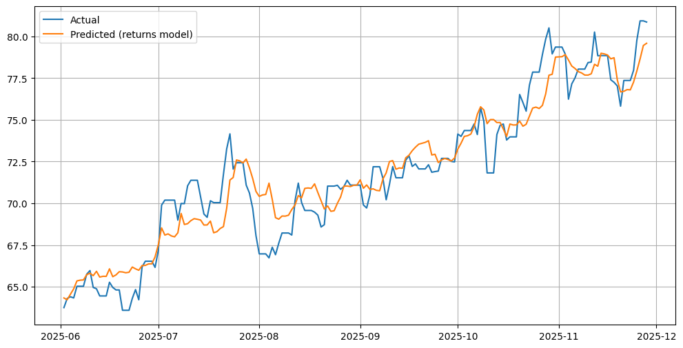
Finally, I plot the reconstructed predicted price series alongside the actual prices.
This visual comparison shows whether the return-based model is capturing the market trend, its turning points, and—most importantly—whether it can follow the new highs that raw-price tree models fail to predict.
In this case, the returns-based XGBoost performs significantly better in tracking the upward trend.
Conclusion
The goal of this project was to build a reliable daily forecast of steel rebar prices using openly available financial data and a reproducible machine-learning workflow. I wanted to understand not only how different models behave when facing real market dynamics, but also how far a simple feature-engineering pipeline can go before more advanced techniques become necessary. Working with ten years of historical prices gave me a realistic scenario to evaluate, since commodity markets present long trends, sharp reversals, and sudden breaks in regime that challenge most supervised models.
I tested several families of models at the end of this analysis. Tree-based ensembles such as Random Forest and Extra Trees delivered relatively stable predictions but failed to follow upward movements beyond the maximum levels observed in the training data. Boosting models like XGBoost, LightGBM, and Gradient Boosting captured nonlinear patterns more effectively but still flattened out whenever the market reached new highs. Linear Regression surprised me with almost perfect fit, but that result was misleading because the model was implicitly exploiting the smoothness of the price curve rather than learning genuine predictive structure. Prophet focused heavily on seasonality and under-fitted the trend component. Overall, the raw-price models delivered MAE values around 2.4 to 3.2 USD per ton and MAPE values in the 3 to 4 percent range, which is acceptable for a baseline but not compelling for real forecasting.
The turning point came when I reframed the problem in terms of log-returns and trained an XGBoost Regressor on these transformed targets. Modeling relative day-to-day changes rather than absolute price levels allows the model to learn momentum, acceleration, and mean-reversion patterns that are invisible when working directly with raw prices. More importantly, log-returns remove the structural ceiling that tree-based models face when the market breaks into new price territory. By compounding the predicted returns back into price space, the model can follow upward or downward shifts that extend beyond the training range. The error metrics reflected this improvement immediately; the return-based XGBoost achieved the lowest MAE and MAPE in the entire experiment and visually produced the most credible trajectory across the test window.
Looking back, there are several things I could have done differently from the beginning to improve the overall modeling process. A more systematic approach to feature scaling and target transformation would have exposed the weakness of raw-price models earlier. Adding volatility measures, momentum indicators, or macroeconomic signals could also enhance the model’s ability to anticipate trend shifts. Cross-validation schemes designed specifically for time series, such as expanding-window validation, would have offered a more robust view of stability across different forecasting horizons. Lastly, incorporating uncertainty quantification or interval predictions from the start would make the output more useful in practical decision-making.
Despite these opportunities for refinement, the workflow I developed here generalizes naturally to many other forecasting domains that do not have “operational features”. Any variable that evolves over time and carries historical structure can be modeled through similar transformations and feature engineering. This includes estimating daily cash collected for financial operations, predicting stock prices using returns and technical indicators, modeling energy consumption patterns, anticipating demand in supply-chain scenarios, or forecasting cryptocurrency volatility during rapid market cycles. The logic remains the same: stabilize the target, extract meaningful temporal signals, respect the chronology of the data, and select a model that reacts well to both local noise and global shifts.
This first phase gave me a solid foundation, a reproducible pipeline, and a clear view of the modeling challenges involved. In the second part of the project I will operationalize the selected model by packaging it into a production-ready API, allowing external systems or users to request a next-day steel rebar price on demand.

Leave a Reply