If you work in a BI team and you are still creating insights manually using tools like Power BI, or Tableau, stay here, this article might be interesting for you.
Over the last few months, I’ve been very curious about how LLMs can be used to automate business processes. So, in this article, I decided to build something that helped me understand all the steps between AI adoption and being close to what we could call an “agent.” This demo was built from the perspective of my own role. I’ve worked for many years as a BI Manager, and in the last few years my focus has been mostly on extracting, transforming, and presenting data as fast and as simply as possible to Order to cash teams.
However, insight generation is a completely different problem. Building insights takes time, and many times you can’t easily explain them at all levels of granularity. For example, if someone asks you for the variation of open AR compared to last year, you can evaluate it at the business unit level. But the real explanation usually lives one level below. You might need to analyze percentage changes by region, market, team, or even customer.
All of this can be calculated inside a dashboard using matrices, drill-downs, or multiple filters. But in practice, this often means spending hours filtering data, looking at charts, and trying to understand why a number changed, sometimes for a question that was asked just a few hours ago. Finding answers in the data can be exciting, but when you manage dozens of metrics in a large organization, this process becomes very demanding.
So I started asking myself: why not automate this with AI?
In this demo, I tried several approaches until I found something I felt comfortable with.
- First, I built simple “flags” directly inside Power BI, using summary tables. These flags represent trends or variations, and I passed them to chatgpt in my case, using the chatgpt API, to generate insights.
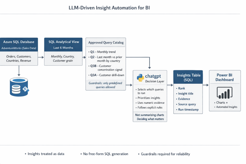
- Then I tried something more advanced. Instead of manually passing flags, I calculated everything directly on top of a SQL view for a specific period. I executed those queries using python, sent the results to chatgpt, generated insights, stored them back in SQL, and finally displayed them inside the dashboard.
- Both approaches worked well, but they had the same limitation: chatgpt was only acting as a narrator. It wasn’t really thinking or deciding anything.
- So I went one step further. I gave to chatgpt a catalog of pre-built SQL queries and asked it to decide which queries to run. Based on the results, it then generated and prioritized the insights.
- There is an even higher level, where the flow SQL → Python → LLM → SQL (Power BI) becomes a loop. In this setup, the system can self-manage within defined limits. For example, it could propose a new query, adjust parameters (like asking for top 20 customers instead of top 12), or explore a different angle. This is where we start talking about a real agent, not just automated insights. I’ll leave that for a future demo.
Although I’ve already explained how the demo works at a high level, I have to say this has been one of the most exhaustive projects I’ve done. I had to find a public sample database from a company called AdventureWorks (a bike retailer), restore it in Azure SQL, configure Azure OpenAI, set up SQL Server Management Studio locally, and configure VS Code with Python and Jupyter to work comfortably.
It was a lot of setup, but it was worth it. This exercise helped me understand how close we already are to implementing an agent-like system without spending thousands of dollars.
In this article, I’ll focus on the following sections. I won’t explain everything in depth, there is already plenty of documentation online about Azure and Power BI and I’ll assume the reader has basic experience with these tools. My goal is to explain the flow and the logic behind the system.
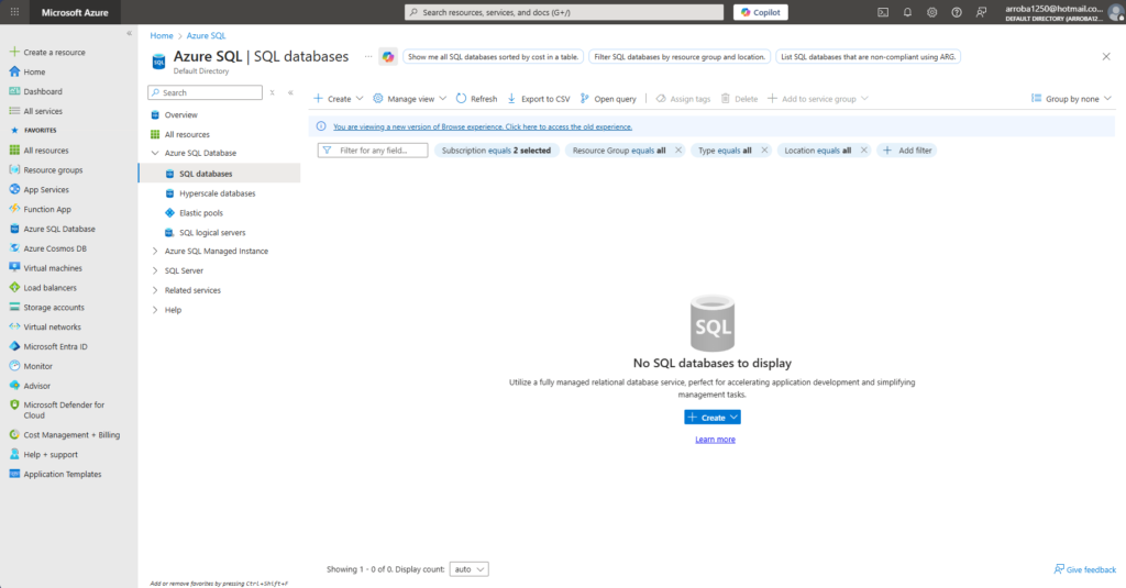
Azure SQL sample database setup
For this demo, I used the AdventureWorks sample database from Microsoft, which represents a bike manufacturing and retail company. I chose it because it has realistic transactional data, customers, territories, and enough complexity to simulate real BI and analytics use cases.
You can download AdventureWorks from Microsoft’s official documentation:
https://learn.microsoft.com/sql/samples/adventureworks-install-configure
At first, I assumed restoring the database into Azure SQL would be straightforward. It wasn’t. AdventureWorks is provided mainly as a .bak backup file, and Azure SQL Database does not support direct restores from .bak files. This was the first issue and something that is not always obvious when coming from a traditional SQL Server background.
Because of this limitation, I had to restore the database locally first using SQL Server Express and SQL Server Management Studio. Once the database was running locally and verified, I then migrated it into Azure SQL Database using the import and migration tools available in Management Studio. This extra step added complexity, but it also reflected a very real scenario when working with cloud-managed databases.
This process alone was a good reminder that Azure SQL is not the same as a full SQL Server instance, and that some operations require different workflows.
Azure SQL Database and Azure OpenAI configuration
After migrating the database, I created a basic Azure SQL Database using the Azure portal, keeping the configuration simple and low-cost since this was only a demo. Once the database was available, I connected to it again through SQL Server Management Studio to validate tables, schemas, and data consistency.
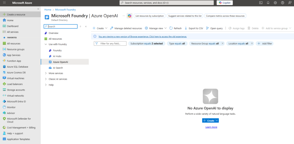
In parallel, I created an Azure OpenAI resource and deployed a chatgpt model. I didn’t focus on advanced configuration here, since the goal of this project was not to explore Azure features in depth, but to understand how chatgpt could be integrated into an analytics workflow.
At this point, the foundation was ready: a transactional dataset running in Azure SQL and a chatgpt deployment available for inference. With this setup in place, I could move to the next step, which was connecting everything using Python and starting to experiment with automated insight generation instead of manual analysis.
Management Studio, VS Code, Jupyter, and Python setup
For this project, I used each tool with a very specific purpose. SQL Server Management Studio was my main interface to Azure SQL. I used it to validate data, explore tables, build and test queries, and later verify the tables where the insights generated by chatgpt were stored.
VS Code was my development environment. I used it to write and organize the Python code that connects SQL Server with chatgpt. Inside VS Code, I worked with Jupyter notebooks to iterate faster, inspect intermediate results, and debug issues without constantly running full scripts.
Python acted as the orchestration layer. It executes SQL queries, prepares structured inputs for chatgpt, receives the generated insights, and inserts them back into the database. This combination allowed me to connect analytics, AI, and visualization into a single workflow without overengineering the setup.
Draft Power BI dashboard for context
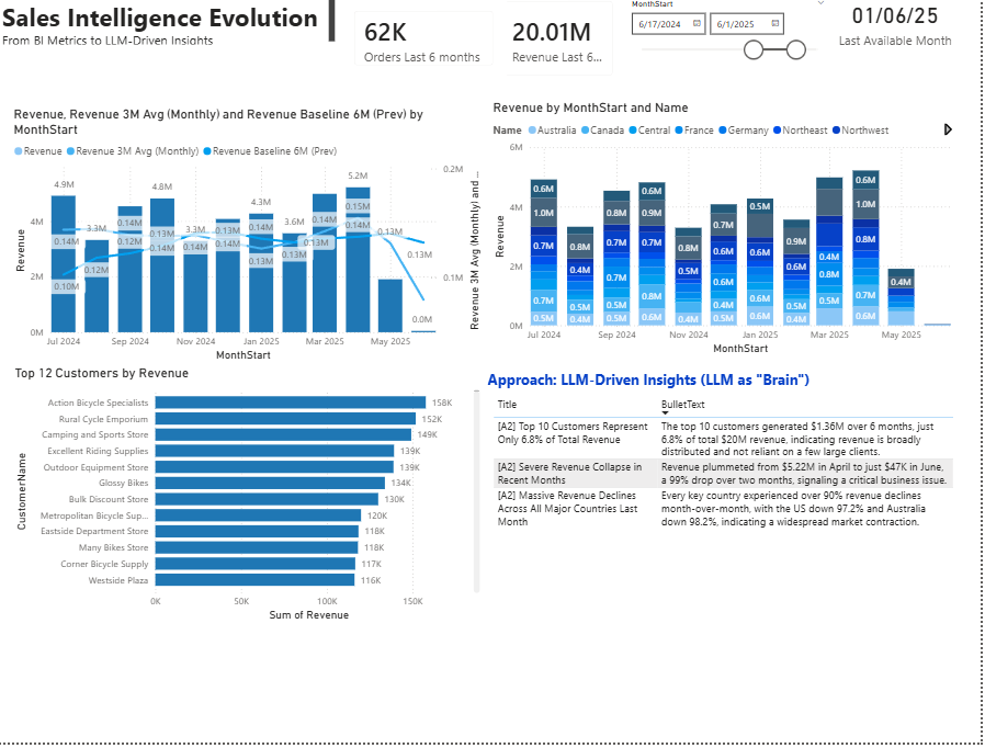
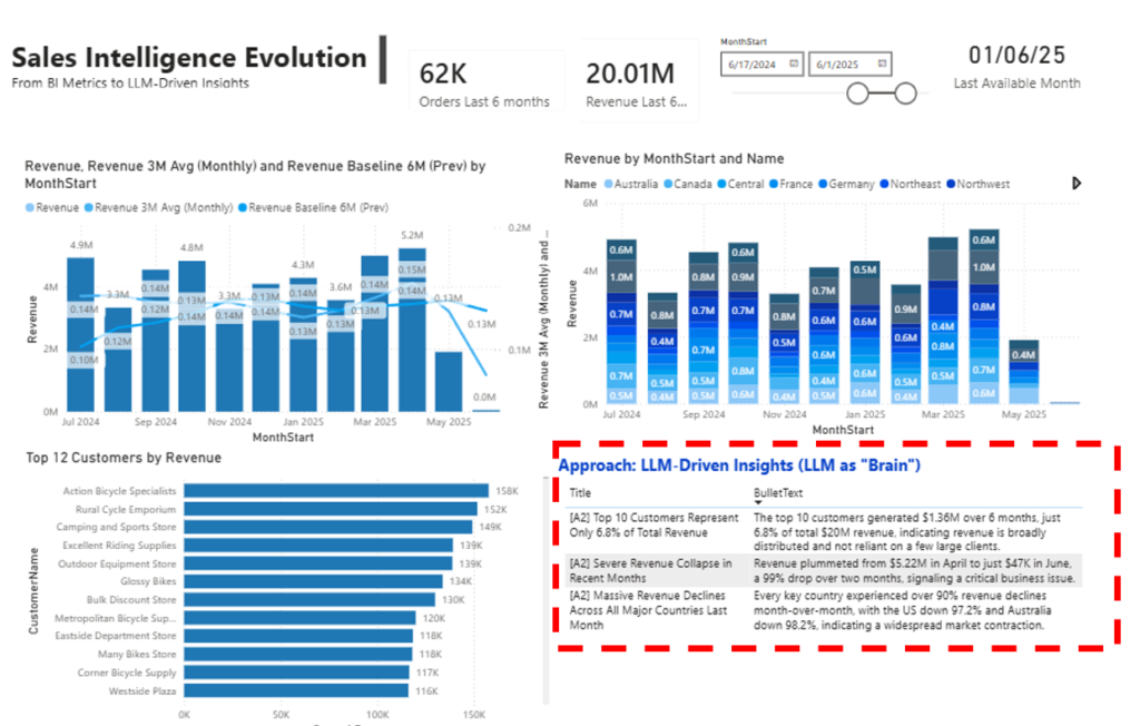
Before generating any automated insights, I built a very simple draft dashboard in Power BI. The goal was not to create a polished executive report, but to provide enough context for the demo. I included three visuals only. First, a revenue trend covering the last 12 months to understand overall direction and seasonality. Second, the same revenue segmented by country, to expose geographic differences. Third, a top 12 customers chart showing the most active accounts by revenue.
I intentionally left June as a likely incomplete month. This was done on purpose, to see whether chatgpt would detect and explain that issue instead of ignoring it or overinterpreting the numbers.
This dashboard is purely explanatory. It exists to support the automation workflow, not to be the final analytical product. The AdventureWorks model contains much more detail and could support deeper analysis, but for this demo, simplicity was key to focus on insight generation rather than visualization complexity.
Why I created a 6-month view before using Python + chatgpt
Before I connected Python with chatgpt, I needed to simplify the data layer. Instead of letting Python join many tables every time, I created a single SQL view that already contains the grain I need for analysis: month, country, customer, and a few key metrics. This makes the workflow cleaner and more repeatable. Python can query one object, receive consistent columns, and send compact outputs to chatgpt without extra transformations. It also helps with governance: the business logic for how I define “last 6 months” and how I aggregate revenue lives in one place in SQL, not scattered across notebooks.
CREATE OR ALTER VIEW dbo.vw_sales_6m_country_customer
AS
-- I first detect the last available month in the data.
-- This makes the view dynamic: it always follows the latest month in SalesOrderHeader.
WITH last_month AS (
    SELECT MAX(EOMONTH(soh.OrderDate)) AS MaxMonthEnd
    FROM Sales.SalesOrderHeader soh
),
base AS (
    SELECT
        -- I normalize dates to MonthStart so I can aggregate cleanly by month.
        MonthStart = DATEFROMPARTS(YEAR(soh.OrderDate), MONTH(soh.OrderDate), 1),

        -- I map each order to a country using Territory -> CountryRegion.
        Country = cr.Name,

        -- I generate a customer name that works for both stores and individual people.
        -- Priority: Store name -> Person full name -> fallback using CustomerID.
        CustomerName = COALESCE(
            st.Name,
            CONCAT(pp.FirstName, ' ', pp.LastName),
            CONCAT('CustomerID ', CAST(soh.CustomerID AS varchar(20)))
        ),

        -- I compute the core metrics I want to analyze:
        -- Orders (distinct orders), Units (qty), and Revenue (LineTotal).
        OrderCount = COUNT(DISTINCT soh.SalesOrderID),
        Units      = SUM(sod.OrderQty),
        Revenue    = SUM(sod.LineTotal)

    FROM Sales.SalesOrderHeader soh
    JOIN Sales.SalesOrderDetail sod
        ON sod.SalesOrderID = soh.SalesOrderID

    JOIN Sales.SalesTerritory t
        ON t.TerritoryID = soh.TerritoryID

    JOIN Person.CountryRegion cr
        ON cr.CountryRegionCode = t.CountryRegionCode

    JOIN Sales.Customer c
        ON c.CustomerID = soh.CustomerID
    LEFT JOIN Sales.Store st
        ON st.BusinessEntityID = c.StoreID
    LEFT JOIN Person.Person pp
        ON pp.BusinessEntityID = c.PersonID

    -- I filter to the last 6 months, based on the last month found above.
    WHERE
        EOMONTH(soh.OrderDate) >= DATEADD(MONTH, -5, (SELECT MaxMonthEnd FROM last_month))

    -- I group at the final grain I want for the project:
    -- MonthStart + Country + CustomerName.
    GROUP BY
        DATEFROMPARTS(YEAR(soh.OrderDate), MONTH(soh.OrderDate), 1),
        cr.Name,
        COALESCE(
            st.Name,
            CONCAT(pp.FirstName, ' ', pp.LastName),
            CONCAT('CustomerID ', CAST(soh.CustomerID AS varchar(20)))
        )
)
-- I expose the clean final dataset for Python and Power BI.
SELECT
    MonthStart, Country, CustomerName, OrderCount, Units, Revenue
FROM base;
GO
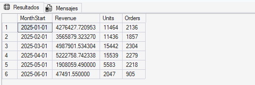
Query 1 — Monthly executive trend (macro)
This query aggregates revenue, units, and orders by month over the last six months. I use it as my “macro lens” because it answers the first question an executive would ask: what is happening overall, month by month? Even if later I go deeper by country or customer, I need this baseline to interpret everything else. A spike or drop is not meaningful unless I can see if it is part of a trend, a seasonality pattern, or a sudden shift. This query also helps validate whether the last month looks incomplete or unusually low compared to prior months. In the workflow, it is usually the first query I want the model to see, because it provides context for interpreting drivers, concentration, and changes.
--Query 1 — Executive trend por mes (macro)
--Aggregates Revenue, Units, and Orders by month for the last 6 months.
--Provides high-level business context to assess overall growth, deceleration, seasonality, and whether recent changes represent a structural shift or a short-term anomaly.

SELECT
  MonthStart,
  Revenue   = SUM(Revenue),
  Units     = SUM(Units),
  Orders    = SUM(OrderCount)
FROM dbo.vw_sales_6m_country_customer
GROUP BY MonthStart
ORDER BY MonthStart;
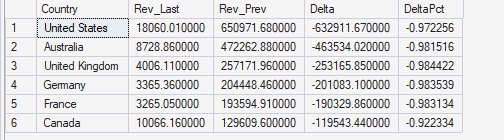
Query 2 — Last month vs prior month revenue drivers (by country)
This query compares the last available month against the previous month, grouped by country. The goal is not to create a full time series by country, but to isolate the most recent movement and identify which geographies contributed the most. I calculate Rev_Last and Rev_Prev and then produce Delta (absolute change) and DeltaPct (percentage change). The reason I focus on Delta and sort by absolute impact is that percent change alone can be misleading when baselines are small. With this query, I can quickly see whether a recent drop or spike is broad-based across multiple countries, or concentrated in one region. In an automated insight workflow, this is a key “driver” query because it helps the model explain the “where” behind the last movement.
-- Query 2: Last month vs prior month revenue drivers (by country)
--Compares last available month revenue against the previous month at country level.
--Identifies which geographies are the primary contributors to the most recent change, prioritizing absolute business impact rather than percentage noise.
WITH m AS (
SELECT
MaxMonth = MAX(MonthStart),
PrevMonth = DATEADD(MONTH, -1, MAX(MonthStart))
FROM dbo.vw_sales_6m_country_customer
),
by_country AS (
SELECT
v.Country,
Rev_Last = SUM(CASE WHEN v.MonthStart = m.MaxMonth THEN v.Revenue ELSE 0 END),
Rev_Prev = SUM(CASE WHEN v.MonthStart = m.PrevMonth THEN v.Revenue ELSE 0 END)
FROM dbo.vw_sales_6m_country_customer v
CROSS JOIN m
GROUP BY v.Country
)
SELECT
Country,
Rev_Last,
Rev_Prev,
Delta = Rev_Last - Rev_Prev,
DeltaPct = CASE WHEN Rev_Prev = 0 THEN NULL ELSE (Rev_Last - Rev_Prev) * 1.0 / Rev_Prev END
FROM by_country
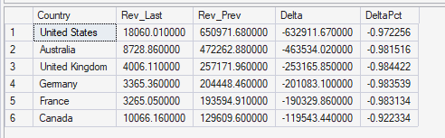
ORDER BY ABS(Rev_Last - Rev_Prev) DESC;Query 2B — Same intent, cleaner handling of DeltaPct edge cases
Query 2B has the same analytical intent as Query 2. It compares last month vs prior month by country and calculates Delta and DeltaPct. The difference is mostly about explicitness and traceability. I wrote it with a more explicit CASE expression for DeltaPct to avoid ambiguity when Rev_Prev is zero (or near zero). In real datasets, some countries may have little or no revenue in the previous month, and percent change can explode or become meaningless. By handling the zero baseline clearly, the output becomes safer to interpret and easier for chatgpt to narrate without producing misleading claims. In practice, I would keep either Query 2 or Query 2B in the catalog, not both, unless I’m testing which format produces more stable outputs for automated insights.
--Query 2B
--Same analytical intent as Query 2, with explicit handling of deltas and percentage change.
--Improves traceability and interpretability of month-over-month movements and avoids ambiguity around zero or near-zero baselines.

WITH m AS (
    SELECT
        MaxMonth  = MAX(MonthStart),
        PrevMonth = DATEADD(MONTH, -1, MAX(MonthStart))
    FROM dbo.vw_sales_6m_country_customer
),
by_country AS (
    SELECT
        v.Country,
        Rev_Last = SUM(CASE WHEN v.MonthStart = m.MaxMonth  THEN v.Revenue ELSE 0 END),
        Rev_Prev = SUM(CASE WHEN v.MonthStart = m.PrevMonth THEN v.Revenue ELSE 0 END)
    FROM dbo.vw_sales_6m_country_customer v
    CROSS JOIN m
    GROUP BY v.Country
)
SELECT
    Country,
    Rev_Last,
    Rev_Prev,
    Delta = Rev_Last - Rev_Prev,
    DeltaPct = CASE
        WHEN Rev_Prev = 0 THEN NULL
        ELSE (Rev_Last - Rev_Prev) * 1.0 / Rev_Prev
    END
FROM by_country
ORDER BY ABS(Rev_Last - Rev_Prev) DESC;
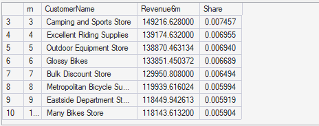
Query 3A — Top 10 customers and their 6-month share
This query ranks the top 10 customers by total revenue over the six-month window and calculates each customer’s share of total revenue. This is the “concentration lens.” It helps answer questions like: do we depend on a small number of customers, or is revenue diversified? It is also useful for prioritization: if a few customers represent a meaningful share, then any change in their purchasing patterns matters more. For automated insights, this is a strong signal because it is interpretable and executive-friendly. It also complements Query 1 and Query 2: even if revenue is dropping overall, executives want to know whether the decline is tied to key accounts or spread across the base. The share metric makes the output actionable, not just descriptive.
-- Query 3A: Top 10 customers + share del total 6m
--Ranks the top 10 customers by cumulative 6-month revenue and calculates each customer’s share of total revenue.
--Used to assess revenue concentration, key account dependency, and potential risk or focus opportunities.
WITH t AS (
    SELECT
        CustomerName,
        Revenue6m = SUM(Revenue)
    FROM dbo.vw_sales_6m_country_customer
    GROUP BY CustomerName
),
tot AS (
    SELECT TotalRev = SUM(Revenue6m) FROM t
),
ranked AS (
    SELECT
        t.CustomerName,
        t.Revenue6m,
        Share = t.Revenue6m * 1.0 / tot.TotalRev,
        rn = ROW_NUMBER() OVER (ORDER BY t.Revenue6m DESC)
    FROM t
    CROSS JOIN tot
)
SELECT
    rn,
    CustomerName,
    Revenue6m,
    Share
FROM ranked
WHERE rn <= 10
ORDER BY rn;
Query 3B — Executive summary of Top 10 concentration
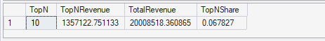
Query 3B takes the same idea as Query 3A but collapses it into a single executive-level summary. Instead of listing customers, it calculates total revenue for the top 10 customers, total revenue overall, and the top-10 share. The point is to produce one simple, high-signal indicator that can be used as a headline insight: “Top 10 customers represent X% of revenue.” This is especially useful when I want chatgpt to prioritize insights without being overwhelmed by too much detail. It also works well as a guardrail-friendly input because it is simple and less prone to misinterpretation. Then, if the model decides concentration is important, it can request Query 3A as a follow-up to name the customers and provide more concrete evidence.
-- Query 3B: Resumen concentración Top10
--Summarizes the combined impact of the Top 10 customers, including total Top-10 revenue, total revenue, and overall Top-10 share.
--Provides a single executive-level signal indicating whether revenue is concentrated or broadly diversified.

WITH t AS (
    SELECT CustomerName, Revenue6m = SUM(Revenue)
    FROM dbo.vw_sales_6m_country_customer
    GROUP BY CustomerName
),
tot AS (
    SELECT TotalRev = SUM(Revenue6m) FROM t
),
ranked AS (
    SELECT
        CustomerName,
        Revenue6m,
        rn = ROW_NUMBER() OVER (ORDER BY Revenue6m DESC)
    FROM t
)
SELECT
    TopN = 10,
    TopNRevenue = SUM(CASE WHEN rn <= 10 THEN Revenue6m ELSE 0 END),
    TotalRevenue = (SELECT TotalRev FROM tot),
    TopNShare = SUM(CASE WHEN rn <= 10 THEN Revenue6m ELSE 0 END) * 1.0 / (SELECT TotalRev FROM tot)
FROM ranked;
Python as the orchestration layer for automated insights
At this stage of the project, Python becomes the central orchestration layer. Its role is not to replace SQL, Power BI, or chatgpt, but to connect them in a controlled and repeatable way. Instead of manually querying data, interpreting charts, and writing insights, Python coordinates each step of the workflow from data extraction to insight persistence.
The first thing I do in Python is load all configuration through environment variables. This includes Azure SQL credentials and the chatgpt deployment details. I intentionally avoid hardcoding any secrets in the script. This makes the setup safer, portable, and closer to how this would work in a real environment.
pip install openai pyodbc pandas
import os

# Azure OpenAI
os.environ["AZURE_OPENAI_ENDPOINT"] = "https://adventure.openai.azure.com/"
os.environ["AZURE_OPENAI_KEY"] = "KEY"
os.environ["AZURE_OPENAI_DEPLOYMENT"] = "gpt-4.1-mini"  # tu deployment name

# Azure SQL (SQL Auth)
os.environ["SQL_SERVER"] = "adventures.database.windows.net"
os.environ["SQL_DB"] = "AdventureWorks2025"
os.environ["SQL_USER"] = "SQLUSER"
os.environ["SQL_PASS"] = "SQLPASSWORD"
Step 1: Planning what to analyze (decision before execution)
Before running any SQL query, I ask chatgpt to create a query plan. Instead of letting it explore data freely, I give it a fixed catalog of approved queries. Each query represents a specific analytical perspective: macro trends, recent drivers, or customer concentration.
At this point, chatgpt is not generating insights yet. Its only task is to decide which queries are worth running, given the goal of producing executive-level insights for the last six months. I limit the number of queries it can choose. This acts as a guardrail and forces prioritization. In practice, this mimics how a human analyst decides what to look at first before diving into details.
This planning step is critical. It shifts the model from being a narrator to being a selector, which is a key step toward agent-like behavior.
Step 2: Executing only approved queries
Once the plan is defined, Python executes only the selected queries against Azure SQL. There is no dynamic SQL generation at this stage. Every query must exist in the approved catalog. This ensures safety, traceability, and consistency.
The query outputs are loaded into pandas DataFrames and then converted into compact, JSON-safe structures. I intentionally limit the number of rows sent to chatgpt to keep payloads small and focused. The goal is to provide enough evidence for reasoning, not to dump raw tables.
At the same time, Python derives the analysis period directly from the query outputs. This avoids hardcoding dates and ensures the insights always reflect the actual data window.
Step 3: Generating ranked executive insights
With all query results prepared, Python sends them back to chatgpt for the second step: insight generation. Here, the model receives multiple analytical perspectives at once, along with explicit rules.
These rules are essential. Chatgpt is instructed to use only the provided data, avoid causal claims, cite numeric evidence, and reference the source queries. It must return a small number of ranked insights, ordered by business impact. This forces clarity and prevents generic or overly verbose explanations.
At this stage, chatgpt is no longer summarizing charts. It is prioritizing information in a way that resembles executive reasoning.
Step 4: Persisting insights for BI consumption
The final step is persistence. Python inserts the generated insights into a dedicated SQL table, along with metadata such as run ID, execution time, model name, and analysis period. From this point on, the insights are just another dataset.
Power BI can consume them directly without any additional logic. This is a key design choice: insights are treated as first-class data, not temporary text outputs. This makes the entire process repeatable, auditable, and easy to integrate into existing BI workflows.
This Python workflow replaces a large portion of manual analytical effort without removing control. The system does not invent questions, write SQL freely, or act autonomously. Instead, it operates within clear guardrails, combining deterministic data processing with probabilistic reasoning.
While this is not yet a fully autonomous agent, it is very close. The planning, execution, reasoning, and persistence layers are already in place. What remains is closing the loop, which is exactly where this project is heading next.
import os, json, uuid, datetime as dt
import pandas as pd
import pyodbc
from openai import AzureOpenAI

# ===========
# CONFIG (leer variables por NOMBRE)
# ===========
AZURE_OPENAI_ENDPOINT = os.environ["AZURE_OPENAI_ENDPOINT"]   # ej: https://adventure.openai.azure.com/
AZURE_OPENAI_KEY = os.environ["AZURE_OPENAI_KEY"]
AZURE_OPENAI_DEPLOYMENT = os.environ.get("AZURE_OPENAI_DEPLOYMENT", "gpt-4.1-mini")

SQL_SERVER = os.environ["SQL_SERVER"]      # ej: adventures.database.windows.net
SQL_DB = os.environ["SQL_DB"]              # ej: AdventureWorks2025
SQL_USER = os.environ["SQL_USER"]
SQL_PASS = os.environ["SQL_PASS"]

# ===========
# SQL helpers
# ===========
def get_conn():
    conn_str = (
        "Driver={ODBC Driver 18 for SQL Server};"
        f"Server=tcp:{SQL_SERVER},1433;"
        f"Database={SQL_DB};"
        f"Uid={SQL_USER};Pwd={SQL_PASS};"
        "Encrypt=yes;TrustServerCertificate=no;Connection Timeout=30;"
    )
    return pyodbc.connect(conn_str)

# ===========
# QUERIES
# ===========
SQL_Q1 = """
-- Q1 — Monthly executive trend (macro view)
SELECT
  MonthStart,
  Revenue   = SUM(Revenue),
  Units     = SUM(Units),
  Orders    = SUM(OrderCount)
FROM dbo.vw_sales_6m_country_customer
GROUP BY MonthStart
ORDER BY MonthStart;
"""

SQL_Q2 = """
-- Q2 — Last month vs prior month revenue drivers (by country)
WITH m AS (
    SELECT
        MaxMonth  = MAX(MonthStart),
        PrevMonth = DATEADD(MONTH, -1, MAX(MonthStart))
    FROM dbo.vw_sales_6m_country_customer
),
by_country AS (
    SELECT
        v.Country,
        Rev_Last = SUM(CASE WHEN v.MonthStart = m.MaxMonth  THEN v.Revenue ELSE 0 END),
        Rev_Prev = SUM(CASE WHEN v.MonthStart = m.PrevMonth THEN v.Revenue ELSE 0 END)
    FROM dbo.vw_sales_6m_country_customer v
    CROSS JOIN m
    GROUP BY v.Country
)
SELECT
    Country,
    Rev_Last,
    Rev_Prev,
    Delta = Rev_Last - Rev_Prev,
    DeltaPct = CASE WHEN Rev_Prev = 0 THEN NULL ELSE (Rev_Last - Rev_Prev) * 1.0 / Rev_Prev END
FROM by_country
ORDER BY ABS(Rev_Last - Rev_Prev) DESC;
"""

SQL_Q3A = """
-- Q3A — Top 10 customers and 6-month revenue share
WITH t AS (
    SELECT
        CustomerName,
        Revenue6m = SUM(Revenue)
    FROM dbo.vw_sales_6m_country_customer
    GROUP BY CustomerName
),
tot AS (
    SELECT TotalRev = SUM(Revenue6m) FROM t
),
ranked AS (
    SELECT
        t.CustomerName,
        t.Revenue6m,
        Share = t.Revenue6m * 1.0 / tot.TotalRev,
        rn = ROW_NUMBER() OVER (ORDER BY t.Revenue6m DESC)
    FROM t
    CROSS JOIN tot
)
SELECT
    rn,
    CustomerName,
    Revenue6m,
    Share
FROM ranked
WHERE rn <= 10
ORDER BY rn;
"""

SQL_Q3B = """
-- Q3B — Top 10 revenue concentration summary
WITH t AS (
    SELECT CustomerName, Revenue6m = SUM(Revenue)
    FROM dbo.vw_sales_6m_country_customer
    GROUP BY CustomerName
),
tot AS (
    SELECT TotalRev = SUM(Revenue6m) FROM t
),
ranked AS (
    SELECT
        CustomerName,
        Revenue6m,
        rn = ROW_NUMBER() OVER (ORDER BY Revenue6m DESC)
    FROM t
)
SELECT
    TopN = 10,
    TopNRevenue = SUM(CASE WHEN rn <= 10 THEN Revenue6m ELSE 0 END),
    TotalRevenue = (SELECT TotalRev FROM tot),
    TopNShare = SUM(CASE WHEN rn <= 10 THEN Revenue6m ELSE 0 END) * 1.0 / (SELECT TotalRev FROM tot)
FROM ranked;
"""

QUERY_CATALOG = {
    "Q1": {"sql": SQL_Q1,  "desc": "Monthly executive trend (Revenue, Units, Orders) for last 6 months."},
    "Q2": {"sql": SQL_Q2,  "desc": "Last month vs prior month revenue drivers by country (Rev_Last, Rev_Prev, Delta, DeltaPct)."},
    "Q3A": {"sql": SQL_Q3A,"desc": "Top 10 customers by 6-month revenue and share of total."},
    "Q3B": {"sql": SQL_Q3B,"desc": "Top 10 customer concentration summary (TopNRevenue, TotalRevenue, TopNShare)."},
}

# ===========
# INSERT
# ===========
INSERT_SQL = """
INSERT INTO dbo.insights_llm_demo
(RunId, RunAt, PeriodStart, PeriodEnd, BulletRank, Title, BulletText, Evidence, Model, Deployment)
VALUES (?, ?, ?, ?, ?, ?, ?, ?, ?, ?);
"""

# ===========
# LLM client
# ===========
client = AzureOpenAI(
    azure_endpoint=AZURE_OPENAI_ENDPOINT,
    api_key=AZURE_OPENAI_KEY,
    api_version="2024-12-01-preview"
)

SYSTEM_PLAN = (
    "You are an analytics agent. You must select which SQL queries to run from the allowed catalog. "
    "Goal: generate executive insights for the last 6 months with the highest business impact. "
    "Constraints: choose up to 3 queries for initial scan, then up to 1 follow-up query. "
    "Prefer including Q1 (macro trend) unless there is a strong reason not to. "
    "Return ONLY JSON."
)

SYSTEM_INSIGHTS = (
    "You are the decision brain for Sales Intelligence. "
    "You will receive outputs from multiple analytical queries. "
    "Your job is to PRIORITIZE what matters most to an executive. "
    "Return 3 to 5 insights ranked by business impact. "
    "Each insight MUST cite numeric evidence and MUST reference the source query (Q1/Q2/Q3A/Q3B). "
    "Do NOT invent causes; only describe what the data shows and why it matters."
)

# ===========
# Output schemas
# ===========
INSIGHTS_SCHEMA = {
  "type": "object",
  "properties": {
    "period_start": {"type": "string"},
    "period_end": {"type": "string"},
    "insights": {
      "type": "array",
      "minItems": 3,
      "maxItems": 5,
      "items": {
        "type": "object",
        "properties": {
          "rank": {"type": "integer"},
          "title": {"type": "string"},
          "bullet": {"type": "string"},
          "evidence": {"type": "string"}
        },
        "required": ["rank", "title", "bullet", "evidence"]
      }
    }
  },
  "required": ["period_start", "period_end", "insights"]
}

PLAN_SCHEMA = {
  "type": "object",
  "properties": {
    "initial_queries": {
      "type": "array",
      "minItems": 1,
      "maxItems": 3,
      "items": {"type": "string", "enum": list(QUERY_CATALOG.keys())}
    },
    "followup_queries": {
      "type": "array",
      "minItems": 0,
      "maxItems": 1,
      "items": {"type": "string", "enum": list(QUERY_CATALOG.keys())}
    },
    "rationale": {"type": "string"}
  },
  "required": ["initial_queries", "followup_queries", "rationale"]
}

# ===========
# Helpers: safe JSON + allowlisted execution
# ===========
def _to_jsonable(val):
    import datetime as _dt
    import decimal as _dec
    import pandas as _pd

    if isinstance(val, (_dt.date, _dt.datetime)):
        return val.isoformat()
    if isinstance(val, _pd.Timestamp):
        return val.to_pydatetime().isoformat()
    if isinstance(val, _dec.Decimal):
        return float(val)
    return val

def df_to_records_jsonable(df: pd.DataFrame, max_rows: int = 200):
    df2 = df.head(max_rows).copy()
    for c in df2.columns:
        df2[c] = df2[c].map(_to_jsonable)
    return df2.to_dict(orient="records")

def run_query(conn, qid: str) -> pd.DataFrame:
    if qid not in QUERY_CATALOG:
        raise ValueError(f"Query not allowed: {qid}")
    return pd.read_sql(QUERY_CATALOG[qid]["sql"], conn)

def dedupe_keep_order(items):
    seen = set()
    out = []
    for x in items:
        if x not in seen:
            seen.add(x)
            out.append(x)
    return out

def derive_period_from_outputs(outputs: dict) -> tuple[str, str]:
    # Prefer Q1 MonthStart (it’s the macro trend)
    if "Q1" in outputs and outputs["Q1"]:
        row0 = outputs["Q1"][0]
        if "MonthStart" in row0:
            ms = [r["MonthStart"] for r in outputs["Q1"] if r.get("MonthStart") is not None]
            if ms:
                return str(min(ms)), str(max(ms))

    # Fallback: search any output with MonthStart
    for _, rows in outputs.items():
        if rows and "MonthStart" in rows[0]:
            ms = [r["MonthStart"] for r in rows if r.get("MonthStart") is not None]
            if ms:
                return str(min(ms)), str(max(ms))

    return "unknown", "unknown"

# ===========
# Main
# ===========
def main():
    run_id = uuid.uuid4()
    run_at = dt.datetime.utcnow().replace(microsecond=0)

    APPROACH_TAG = "A3"  # agent version
    MODEL_NAME = AZURE_OPENAI_DEPLOYMENT

    # ----------------
    # 1) PLAN: LLM selects queries
    # ----------------
    catalog_for_model = [{"id": k, "description": v["desc"]} for k, v in QUERY_CATALOG.items()]

    plan_msg = {
        "goal": "Generate 3-5 executive insights for the last 6 months using the best available queries.",
        "allowed_queries": catalog_for_model,
        "constraints": {"initial_max": 3, "followup_max": 1},
        "notes": [
            "Prefer Q1 for context.",
            "Avoid redundant queries unless needed for validation."
        ]
    }

    plan_resp = client.chat.completions.create(
        model=AZURE_OPENAI_DEPLOYMENT,
        temperature=0.1,
        messages=[
            {"role": "system", "content": SYSTEM_PLAN},
            {"role": "user", "content": json.dumps(plan_msg, ensure_ascii=False)}
        ],
        response_format={
            "type": "json_schema",
            "json_schema": {"name": "query_plan", "schema": PLAN_SCHEMA}
        }
    )

    plan = json.loads(plan_resp.choices[0].message.content)
    chosen_qs = dedupe_keep_order(plan["initial_queries"] + plan["followup_queries"])

    # Guardrail: never run more than 4 total
    chosen_qs = chosen_qs[:4]

    # ----------------
    # 2) EXECUTE: run only selected allowlisted queries
    # ----------------
    outputs = {}
    with get_conn() as conn:
        for qid in chosen_qs:
            df = run_query(conn, qid)
            outputs[qid] = df_to_records_jsonable(df, max_rows=200)

    period_start, period_end = derive_period_from_outputs(outputs)

    # ----------------
    # 3) INSIGHTS: generate final bullets
    # ----------------
    insights_msg = {
        "period_start": period_start,
        "period_end": period_end,
        "query_plan": plan,
        "queries_executed": chosen_qs,
        "query_outputs": outputs,
        "rules": [
            "Use only provided data.",
            "No causal claims without evidence.",
            "Every insight must include numbers and reference at least one source query (Q1/Q2/Q3A/Q3B).",
            "Evidence must include a 'Sources:' tag like 'Sources: Q1,Q2'.",
            "Prioritize impact: what an exec should care about first."
        ]
    }

    resp = client.chat.completions.create(
        model=AZURE_OPENAI_DEPLOYMENT,
        temperature=0.2,
        messages=[
            {"role": "system", "content": SYSTEM_INSIGHTS},
            {"role": "user", "content": json.dumps(insights_msg, ensure_ascii=False)}
        ],
        response_format={
            "type": "json_schema",
            "json_schema": {"name": "exec_insights", "schema": INSIGHTS_SCHEMA}
        }
    )

    out = json.loads(resp.choices[0].message.content)

    # ----------------
    # 4) INSERT results into SQL
    # ----------------
    with get_conn() as conn:
        cur = conn.cursor()
        for ins in out["insights"]:
            cur.execute(
                INSERT_SQL,
                str(run_id),
                run_at,
                out["period_start"],
                out["period_end"],
                int(ins["rank"]),
                f"[{APPROACH_TAG}] {ins['title']}"[:200],
                ins["bullet"],
                ins.get("evidence"),
                MODEL_NAME,
                f"{AZURE_OPENAI_DEPLOYMENT}-{APPROACH_TAG}"
            )
        conn.commit()

    print("OK. Inserted insights:", len(out["insights"]), "RunId:", run_id)
    print("Plan:", chosen_qs)
    print("Rationale:", plan.get("rationale"))

if __name__ == "__main__":
    main()
Project conclusion
The goal of this project was to test whether part of the insight work that BI teams usually do manually can be automated using chatgpt, without turning this into a complex or overengineered solution. Instead of focusing on perfect dashboards or advanced models, I focused on connecting SQL, Python, chatgpt, and Power BI into a workflow where insights are generated, stored, and displayed automatically.
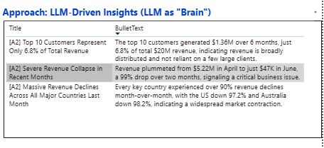
When I look at the dashboard together with the insights generated, the logic is consistent and easy to follow. The system first rules out customer concentration as a root cause. Based on the data, the top 10 customers represent only 6.8% of total six-month revenue. That immediately tells us that the business is not dependent on a few large clients, so this is not the area to investigate further. This is a good example of how an automated insight can help narrow the search space instead of adding noise.
Next, the model focuses on the most visible anomaly in the charts: a sharp drop in revenue in the most recent month. From the model’s point of view, this is the highest-impact signal, so it surfaces it as the top insight. When it then looks at revenue by country, it reinforces the same narrative. The decline appears across all major regions, not just one market, which strengthens the idea of a systemic issue rather than a localized problem.
This is where the most important learning appears. Chatgpt correctly detected that something unusual happened in June, but it assumed the drop was a real business collapse. It did not question whether the month might be incomplete. That was intentional in this demo. I did not provide an explicit data freshness or completeness signal, and the model behaved exactly as expected: it explained the numbers it was given. This is not a model failure. It is a design lesson. Automated insights are only as good as the guardrails we define.
From a project perspective, the biggest takeaway is that meaningful insight automation does not require complex machine learning. Most of the value came from good SQL, a small set of well-defined queries, and forcing the model to prioritize instead of narrate everything. Python simply orchestrated the flow and made the process repeatable.
If I were to improve this demo using the same tools, the first step would be to add explicit signals for data completeness and freshness, so the model can distinguish between real business issues and data artifacts. That alone would significantly improve the quality of the insights.
At an enterprise level, the challenge is not technology but ownership. BI teams would own the data models and approved queries, while data science or advanced analytics teams would own the reasoning layer and guardrails. When both work together, dashboards stop being static reports and start becoming systems that actively surface what matters.
In short, this demo shows that we are already very close to automating insights, but it also shows that the real intelligence is not in the model alone, but in how we frame the problem and control the reasoning.
Leave a Reply